Model specification
This section continues on from the end of the previous section on exploratory data analysis.
Taking everything that we have seen so far, we will initially specify our model without any interaction and polynomial terms: \[ \begin{aligned} \log(wage_i) &= \beta_0 + \beta_1 educ_i + \beta_2 exper_i + \beta_3 metro_i + \\ &+ \beta_4 south_i + \beta_5 west_i + \beta_6 midwest_i \\ &+ \beta_7 female_i + \beta_{8} black_i + \epsilon_i,\quad i = 1,...,N \end{aligned} \]
We expect the following signs for the non-intercept coefficients:
-
\(\beta_1 > 0\) - additional years of education should increase the hourly
wage; -
\(\beta_2 > 0\) - additional years of experience should increase the hourly
wage; - \(\beta_3 > 0\) - a metropolitan is a highly dense population area. Generally, businesses are located in such high-density areas, and competition is higher. Consequently, we would expect someone from a metropolitan area to earn more than someone else, from the less-populated areas.
- \(\beta_4, \beta_5, \beta_6\) - we are not sure of the sign as of yet. The region may also be correlated with the metropolitan indicator variable, as some regions could be less populated.
- \(\beta_7, \beta_{8}\) - we are interested in evaluating if there is discrimination in the workforce (in which case these variables would be negative). Though it is important to note - as we will later see - the model may exhibit all sorts of problems - multicollinearity, autocorrelation, heteroskedasticity - which would result in biased and/or insignificant coefficients. If our goal is to evaluate the effect - we should be careful that our model is correctly specified!
- We assume that other family income,
faminc, should not affect the wage of a person, i.e. we treat it as an insignificant variable, whose correlation may be spurious and as such, we do not include it in the model.
The sign expectations are not based on the data, but rather on the definitions of these variables and how we expect them to affect \(wage\) (based on economic theory).
We will also estimate two additional models in order to showcase the effect of taking logarithms: \[ \begin{aligned} wage_i &= \beta_0 + \beta_1 \cdot educ_i + \varepsilon_i \quad \mbox{(a simple linear model)} \\ \log(wage_i) &= \beta_0 + \beta_1 \cdot educ_i + \varepsilon_i \quad \mbox{(a log-linear model)} \end{aligned} \]
mdl_small_1 = smf.ols(formula = "wage ~ 1 + educ", data = dt_train).fit()
mdl_small_2 = smf.ols(formula = "np.log(wage) ~ 1 + educ", data = dt_train).fit()
Call:
lm(formula = "wage ~ educ", data = dt_train)

Residuals:
    Min      1Q  Median      3Q     Max
-31.143  -8.361  -3.302   5.991  71.373

Coefficients:
            Estimate Std. Error t value Pr(>|t|)
(Intercept)  -9.4359     1.9705  -4.788 1.95e-06 ***
educ          2.3164     0.1361  17.025  < 2e-16 ***
---
Signif. codes:  0 '***' 0.001 '**' 0.01 '*' 0.05 '.' 0.1 ' ' 1

Residual standard error: 12.28 on 958 degrees of freedom
Multiple R-squared:  0.2323,    Adjusted R-squared:  0.2315
F-statistic: 289.8 on 1 and 958 DF, p-value: < 2.2e-16print(mdl_small_1.summary()) OLS Regression Results
==============================================================================
Dep. Variable: wage R-squared: 0.232
Model: OLS Adj. R-squared: 0.231
Method: Least Squares F-statistic: 289.8
Date: Mon, 15 Apr 2024 Prob (F-statistic): 5.50e-57
Time: 04:22:28 Log-Likelihood: -3769.0
No. Observations: 960 AIC: 7542.
Df Residuals: 958 BIC: 7552.
Df Model: 1
Covariance Type: nonrobust
==============================================================================
coef std err t P>|t| [0.025 0.975]
------------------------------------------------------------------------------
Intercept -9.4359 1.971 -4.788 0.000 -13.303 -5.569
educ 2.3164 0.136 17.025 0.000 2.049 2.583
==============================================================================
Omnibus: 204.972 Durbin-Watson: 1.981
Prob(Omnibus): 0.000 Jarque-Bera (JB): 414.661
Skew: 1.216 Prob(JB): 9.07e-91
Kurtosis: 5.109 Cond. No. 72.3
==============================================================================
Notes:
[1] Standard Errors assume that the covariance matrix of the errors is correctly specified.
Call:
lm(formula = "log(wage) ~ educ", data = dt_train)

Residuals:
     Min       1Q   Median       3Q      Max
-1.80900 -0.32924 -0.01473  0.33719  1.42350

Coefficients:
            Estimate Std. Error t value Pr(>|t|)
(Intercept) 1.625299   0.077090   21.08   <2e-16 ***
educ        0.096645   0.005323   18.16   <2e-16 ***
---
Signif. codes:  0 '***' 0.001 '**' 0.01 '*' 0.05 '.' 0.1 ' ' 1

Residual standard error: 0.4805 on 958 degrees of freedom
Multiple R-squared:  0.256, Adjusted R-squared:  0.2552
F-statistic: 329.6 on 1 and 958 DF, p-value: < 2.2e-16print(mdl_small_2.summary()) OLS Regression Results
==============================================================================
Dep. Variable: np.log(wage) R-squared: 0.256
Model: OLS Adj. R-squared: 0.255
Method: Least Squares F-statistic: 329.6
Date: Mon, 15 Apr 2024 Prob (F-statistic): 1.54e-63
Time: 04:22:29 Log-Likelihood: -657.52
No. Observations: 960 AIC: 1319.
Df Residuals: 958 BIC: 1329.
Df Model: 1
Covariance Type: nonrobust
==============================================================================
coef std err t P>|t| [0.025 0.975]
------------------------------------------------------------------------------
Intercept 1.6253 0.077 21.083 0.000 1.474 1.777
educ 0.0966 0.005 18.156 0.000 0.086 0.107
==============================================================================
Omnibus: 1.860 Durbin-Watson: 1.988
Prob(Omnibus): 0.395 Jarque-Bera (JB): 1.727
Skew: 0.006 Prob(JB): 0.422
Kurtosis: 2.793 Cond. No. 72.3
==============================================================================
Notes:
[1] Standard Errors assume that the covariance matrix of the errors is correctly specified.The estimated models are: \[ \begin{aligned} \widehat{wage}_i &= -9.44 + 2.32 \cdot educ_i \\ \widehat{\log(wage_i)} &= 1.63 + 0.097 \cdot educ_i \end{aligned} \] The interpretation of the coefficients of these models is as follows:
For the simple linear model (also called the level-level model), the intuition on the interpretation is as follows: \[
\dfrac{\partial \widehat{wage}_i}{\partial educ_i} = 2.32
\] We know that educ is measured in years and wage is measured in \(\$/hour\), so an additional year increase in educ (i.e. a unit increase in \(X\)) results in a \(2.32\) increase hourly wage wage (i.e. the unit change in \(Y\)).
Alternatively, we can simply calculate the difference between a regression with \(educ_i\), \(\widehat{wage}_i^{(0)}\) and one with \(educ_i + 1\), \(\widehat{wage}_i^{(1)}\): \[ \widehat{wage}_i^{(1)} - \widehat{wage}_i^{(0)} = -9.44 + 2.32 \cdot (educ_i+1) - (-9.44 + 2.32 \cdot educ_i) = 2.32 \]
For the log-linear model, the interpretation is slightly different. For small changes in \(Y\), it can be shown that: \[
\Delta \log(Y) = \log(Y^{(1)}/Y^{(0)})= \log(Y^{(1)}) - \log(Y^{(0)}) \approx \dfrac{Y^{(1)}-Y^{(0)}}{Y^{(0)}} = \dfrac{\Delta Y}{Y^{(0)}}
\] Then, a percentage change in \(Y\), from \(Y^{(0)}\) to \(Y^{(1)}\) is defined as the log difference, multiplied by \(100\): \[
\% \Delta Y \approx 100 \cdot \Delta \log(Y)
\] In our case, we have that: \[
\dfrac{\partial \log(wage_i)}{\partial educ_i} = 0.097
\] So, if education, educ increase by one year, then hourly wage increases by \(100\cdot 0.097=9.7\%\).
However, the above is only valid of \(Y >0\) is small (e.g. \(Y \in [0.01, \dots, 0.1]\)), since then \(\log(1+Y)\approx Y\). This approximation deteriorates as \(Y\) gets larger, e.g.:
If we exponentiate our log-linear model, then: \[
\widehat{wage}_i = \exp(1.63 + 0.097 \cdot educ_i) = \exp(1.63) \cdot \exp(0.097 \cdot educ_i)
\] Then, a percentage change in wage can be calculated as: \[
\begin{aligned}
100 \cdot \dfrac{\widehat{wage}_i^{(1)} - \widehat{wage}_i^{(0)}}{\widehat{wage}_i^{(0)}} &=
100 \cdot \left(\dfrac{\widehat{wage}_i^{(1)}}{\widehat{wage}_i^{(0)}} - 1 \right) = 100 \cdot \left(\dfrac{\exp(0.097 \cdot (educ_i+1))}{\exp(0.097 \cdot educ_i)}- 1\right)\\
&= 100 \cdot \left( \dfrac{\exp(0.097 \cdot educ_i)\cdot\exp(0.097)}{\exp(0.097 \cdot educ_i)}- 1\right) \\
&= 100 \cdot (\exp(0.097) - 1)
\end{aligned}
\] which equals:
So, a more accurate interpretation for the log-linear model is that a unit increase in \(X_{j,i}\) results in an \(100\cdot(\exp(\beta_j)-1)\%\) change in \(Y\). In our case - an additional year in educ results in a \(10.15\%\) increase in wage, on average.
Note that:
- for the linear-log model, \(Y_i = \beta_0 + \beta_1 \log(X_i) +\varepsilon_i\), a \(1\%\) increase in \(X\) results in a \(\beta_1/100\) unit change in \(Y\). A \(z\%\) increase in \(X\) result in a \(\beta_1/100 \cdot \log(1+z)\) unit change in \(Y\). E.g. for a \(15\%\) increase in \(X\), the unit change in \(Y\) would be equal to \(\beta_1/100 \cdot\log(1.15)\).
- for the log-log model, \(\log(Y_i) = \beta_0 + \beta_1 \log(X_i) +\varepsilon_i\), a \(1\%\) increase in \(X\) results in a \(\beta_1\) percentage change in \(Y\). A \(z\%\) increase in \(X\) result in a \((\log(1+z)^{\beta_1}-1)\cdot 100\) percentage change in \(Y\).
We can compare \(Y\) with \(\widehat{Y}\) to see some immediate differences between the models:
p4 <- dt_train %>%
  dplyr::select(wage, educ) %>%
  dplyr::mutate(wage_mdl_1 = predict(mdl_small_1),
                wage_mdl_2 = exp(predict(mdl_small_2))) %>%
  ggplot(aes(x = educ)) +
  geom_point(aes(y = wage), color = "cornflowerblue") +
  geom_line(aes(y = wage_mdl_1), color = "red") +
  geom_line(aes(y = wage_mdl_2), color = "darkgreen") +
  geom_hline(yintercept = 0, linetype = "dashed") +
  theme_bw()
print(p4)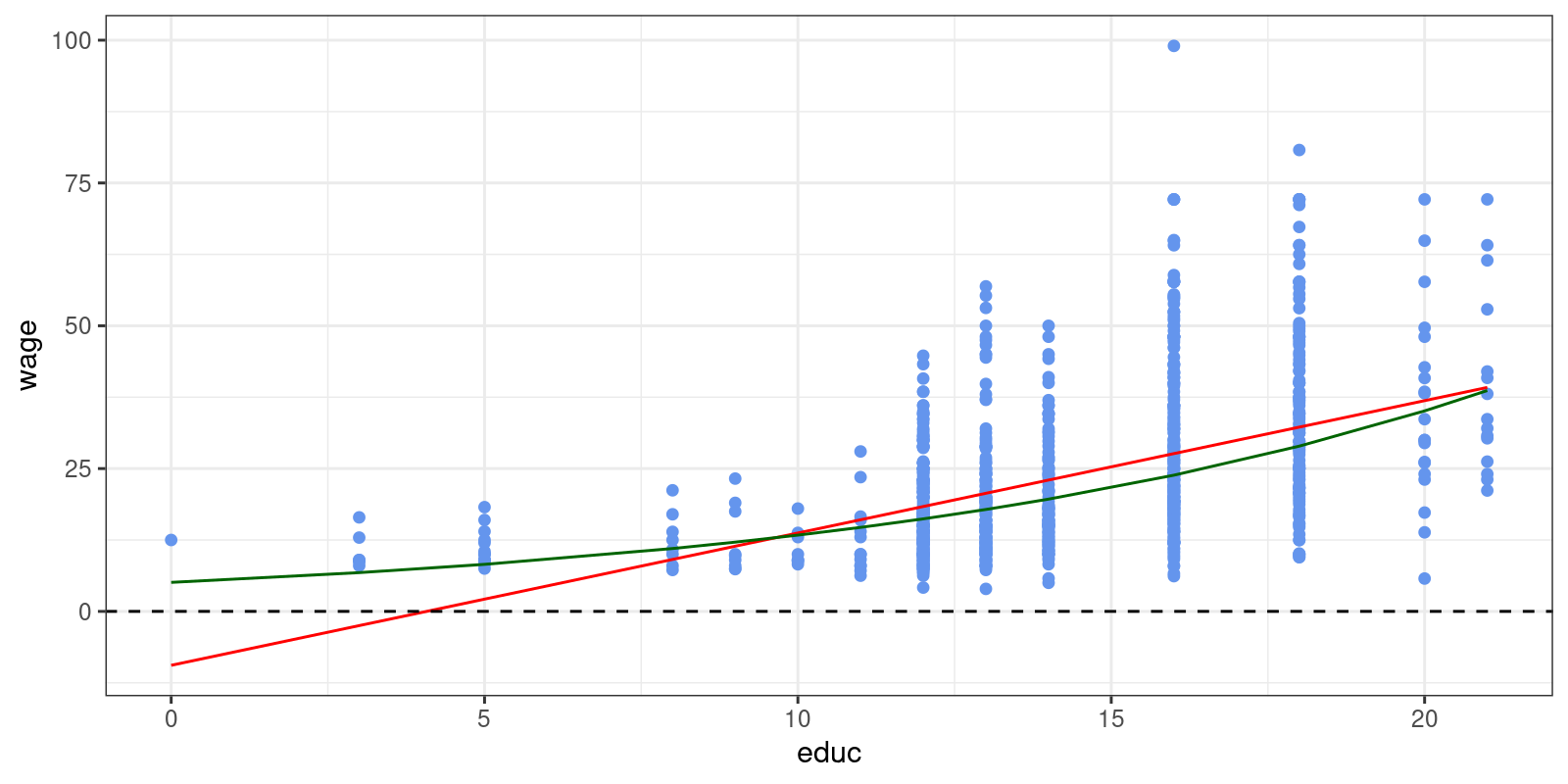
#
p4 = dt_train[["wage", "educ"]].copy()
p4["wage_mdl_1"] = mdl_small_1.predict()
p4["wage_mdl_2"] = np.exp(mdl_small_2.predict())
p4 = (pl.ggplot(data = p4, mapping = pl.aes(x = "educ")) +\
  pl.geom_point(mapping = pl.aes(y = "wage"), color = "cornflowerblue") +\
  pl.geom_line(mapping = pl.aes(y = "wage_mdl_1"), color = "red") +\
  pl.geom_line(mapping = pl.aes(y = "wage_mdl_2"), color = "darkgreen") +\
  pl.geom_hline(yintercept = 0, linetype = "dashed") +\
  pl.theme_bw())
print(p4)
The most notable difference - the log-linear model contains only positive wage values.
Next, we will estimate our specified regression model:
mdl_0 <- lm(formula = "log(wage) ~ educ + exper + metro + south + west + midwest + female + black", data = dt_train)
mdl_0 %>% summary() %>% coef() %>% round(4)
Estimate Std. Error t value Pr(>|t|)
(Intercept) 1.2840 0.0972 13.2102 0.0000
educ 0.1070 0.0053 20.1863 0.0000
exper 0.0086 0.0012 7.4405 0.0000
metro 0.1479 0.0392 3.7758 0.0002
south -0.0998 0.0443 -2.2515 0.0246
west -0.0463 0.0465 -0.9957 0.3196
midwest -0.0487 0.0463 -1.0530 0.2926
female -0.1560 0.0304 -5.1363 0.0000
black -0.0472 0.0566 -0.8350 0.4039mdl_0_spec = smf.ols(formula = "np.log(wage) ~ educ + exper + metro + south + west + midwest + female + black", data = dt_train)
mdl_0 = mdl_0_spec.fit()
print(mdl_0.summary().tables[1])==============================================================================
coef std err t P>|t| [0.025 0.975]
------------------------------------------------------------------------------
Intercept 1.2840 0.097 13.210 0.000 1.093 1.475
educ 0.1070 0.005 20.186 0.000 0.097 0.117
exper 0.0086 0.001 7.440 0.000 0.006 0.011
metro 0.1479 0.039 3.776 0.000 0.071 0.225
south -0.0998 0.044 -2.252 0.025 -0.187 -0.013
west -0.0463 0.046 -0.996 0.320 -0.137 0.045
midwest -0.0487 0.046 -1.053 0.293 -0.140 0.042
female -0.1560 0.030 -5.136 0.000 -0.216 -0.096
black -0.0472 0.057 -0.835 0.404 -0.158 0.064
==============================================================================Compared with our initial assumptions we see that:
-
educ,experandmetrohave a positive effect onwage, as we have expected. - the regional indicator variables
south,westandmidwesthave a negative effect onwage, compared to the base region group. In this case the base group is comprised oneast,northand any other region, which is not covered bysouth,westandmidwestregions. On the other hand, we haven’t yet looked whether these effects are statistically significant. - similarly, gender and race also have negative effects on
wage. However, we will look at their significance in the next section.
Remember, that we have created a geography variable, which we can substitute instead of the separate indicator variables south, west and midwest:
mdl_1 <- lm(formula = "log(wage) ~ educ + exper + metro + geography + female + black", data = dt_train)
mdl_1 %>% summary() %>% coef() %>% round(2)
Estimate Std. Error t value Pr(>|t|)
(Intercept) 1.28 0.10 13.21 0.00
educ 0.11 0.01 20.19 0.00
exper 0.01 0.00 7.44 0.00
metro 0.15 0.04 3.78 0.00
geographysouth -0.10 0.04 -2.25 0.02
geographywest -0.05 0.05 -1.00 0.32
geographymidwest -0.05 0.05 -1.05 0.29
female -0.16 0.03 -5.14 0.00
black -0.05 0.06 -0.84 0.40mdl_1_spec = smf.ols(formula = "np.log(wage) ~ educ + exper + metro + geography + female + black", data = dt_train)
mdl_1 = mdl_1_spec.fit()
print(mdl_1.summary().tables[1])========================================================================================
coef std err t P>|t| [0.025 0.975]
----------------------------------------------------------------------------------------
Intercept 1.2840 0.097 13.210 0.000 1.093 1.475
geography[T.south] -0.0998 0.044 -2.252 0.025 -0.187 -0.013
geography[T.west] -0.0463 0.046 -0.996 0.320 -0.137 0.045
geography[T.midwest] -0.0487 0.046 -1.053 0.293 -0.140 0.042
educ 0.1070 0.005 20.186 0.000 0.097 0.117
exper 0.0086 0.001 7.440 0.000 0.006 0.011
metro 0.1479 0.039 3.776 0.000 0.071 0.225
female -0.1560 0.030 -5.136 0.000 -0.216 -0.096
black -0.0472 0.057 -0.835 0.404 -0.158 0.064
========================================================================================Note the naming for the geography indicator variables is prefixed with the categorical variable name, in order to differentiate, which indicator variables belong to the same categorical variable. Other that that, the coefficients are exactly the same, with the added benefit that we have a single categorical variable in the dataset, instead of multiple columns.
It should be noted that, behind the scenes R and Python automatically creates the indicator variables from these categorical variables. We can verify this by examining the design matrix:
mdl_0 %>% model.matrix() %>% head(5) %>% print() (Intercept) educ exper metro south west midwest female black
1 1 13 45 1 0 1 0 1 0
2 1 14 25 1 0 0 1 1 0
3 1 18 27 1 0 0 0 1 0
4 1 13 42 1 0 0 1 0 0
5 1 13 41 1 0 1 0 1 0mdl_1 %>% model.matrix() %>% head(5) %>% print() (Intercept) educ exper metro geographysouth geographywest geographymidwest female black
1 1 13 45 1 0 1 0 1 0
2 1 14 25 1 0 0 1 1 0
3 1 18 27 1 0 0 0 1 0
4 1 13 42 1 0 0 1 0 0
5 1 13 41 1 0 1 0 1 0print(patsy.dmatrices(mdl_0_spec.formula, data = dt_train, return_type='dataframe')[1].head(5)) Intercept educ exper metro south west midwest female black
0 1.0 13.0 45.0 1.0 0.0 1.0 0.0 1.0 0.0
1 1.0 14.0 25.0 1.0 0.0 0.0 1.0 1.0 0.0
2 1.0 18.0 27.0 1.0 0.0 0.0 0.0 1.0 0.0
3 1.0 13.0 42.0 1.0 0.0 0.0 1.0 0.0 0.0
4 1.0 13.0 41.0 1.0 0.0 1.0 0.0 1.0 0.0print(patsy.dmatrices(mdl_1_spec.formula, data = dt_train, return_type='dataframe')[1].head(5)) Intercept geography[T.south] geography[T.west] geography[T.midwest] educ exper metro female black
0 1.0 0.0 1.0 0.0 13.0 45.0 1.0 1.0 0.0
1 1.0 0.0 0.0 1.0 14.0 25.0 1.0 1.0 0.0
2 1.0 0.0 0.0 0.0 18.0 27.0 1.0 1.0 0.0
3 1.0 0.0 0.0 1.0 13.0 42.0 1.0 0.0 0.0
4 1.0 0.0 1.0 0.0 13.0 41.0 1.0 1.0 0.0