We would expect the following relationship between the independent variables and the participation rate:
\(\beta_{educ}>0\) - a higher education is more likely to lead to an active labor force participation, since the person has already invested their time into improving themselves and have a better chance of earning a higher wage, hence they are more likely to be motivated to return to the workforce; \(\beta_{exper}>0\) - the more experience they have, the more likely that they will return to a higher pay job, hence they are more motivated to return to the workforce; \(\beta_{age}<0\) - the older they are, the less likely they are to be hired back in a good paying position. Hence they may be discouraged from returning to the workforce;
In addition:
\(\beta_{kidslt6}<0\) - the more younger kinds in the family, the higher chance that one of the parents will remain at home to look after them;
\(\beta_{kidsge6}>0\) - older children are at school or daycare, so the parent is less likely to stay at home, when they could be working (especially since buying school supplies, clothes, etc. would benefit from additional income).
glm(inlf~1+educ+exper+age+kidslt6+kidsge6+hours, data =dt_train, family =binomial)%>%summary()
Warning: glm.fit: algorithm did not converge
Warning: glm.fit: fitted probabilities numerically 0 or 1 occurred
Call:
glm(formula = inlf ~ 1 + educ + exper + age + kidslt6 + kidsge6 +
    hours, family = binomial, data = dt_train)

Coefficients:
             Estimate Std. Error z value Pr(>|z|)
(Intercept)  -40.1499  5146.0208  -0.008    0.994
educ           1.0450   185.2361   0.006    0.995
exper         -0.4995   154.3390  -0.003    0.997
age            0.1465    65.7403   0.002    0.998
kidslt6       -0.3265   631.4149  -0.001    1.000
kidsge6        1.5228   333.1617   0.005    0.996
hours          2.2316    45.0036   0.050    0.960

(Dispersion parameter for binomial family taken to be 1)

    Null deviance: 8.2043e+02  on 601  degrees of freedom
Residual deviance: 9.3449e-06  on 595  degrees of freedom
AIC: 14

Number of Fisher Scoring iterations: 25
1
1
Note the high \(p\)-values and warning about convergence - since hours > 0 directly relates to inlf=1 - we get a warning telling us that one of our wariables is able to perfectly separate the different groupr of inlf.
We may want to include the following variables:
\(educ^2\) - each additional year of education would have a decreasing effect on the participation rate, so that \(\beta_{educ^2} < 0\);
\(exper^2\) - each additional year of experience would have a decreasing effect on the participation rate, so that \(\beta_{exper^2} < 0\);
\(age^2\) - each additional year of experience would have an increasing negative effect on the participation rate, so that \(\beta_{age^2}<0\);
\(\rm kidslt6^2\) - each additional young kid would significantly reduce the participation rate further, so that \(\beta_{kidslt6^2}<0\);
\(\rm kidsge6^2\) - each additional older kid would further increase the participation rate, since more money is needed for clothes, books, trips, after school activities, etc. On the other hand, younger children may get hand-me-downs from their older siblings.
Regarding interaction terms, lets assume that we want to include:
\(kidslt6\times kidsge6\) - if we already have a number of older kids, and then we have a younger child, then it may be more likely that the older sibling will babysit the younger ones. Meanwhile the parents can go to work.
my_formula="inlf ~ 1 + educ + I(educ^2) + exper + I(exper^2) + age + kidslt6 + kidsge6 + kidslt6*kidsge6"logit_glm=glm(my_formula, data =dt_train, family =binomial)summary(logit_glm)
Call:
glm(formula = my_formula, family = binomial, data = dt_train)

Coefficients:
                 Estimate Std. Error z value Pr(>|z|)
(Intercept)      5.040155   2.129311   2.367  0.01793 *
educ            -0.530697   0.313145  -1.695  0.09013 .
I(educ^2)        0.030340   0.012822   2.366  0.01797 *
exper            0.199566   0.034957   5.709 1.14e-08 ***
I(exper^2)      -0.003154   0.001104  -2.858  0.00426 **
age             -0.095150   0.016492  -5.770 7.95e-09 ***
kidslt6         -2.174765   0.351711  -6.183 6.27e-10 ***
kidsge6         -0.021683   0.093832  -0.231  0.81725
kidslt6:kidsge6  0.389727   0.139276   2.798  0.00514 **
---
Signif. codes:  0 '***' 0.001 '**' 0.01 '*' 0.05 '.' 0.1 ' ' 1

(Dispersion parameter for binomial family taken to be 1)

    Null deviance: 820.43  on 601  degrees of freedom
Residual deviance: 647.80  on 593  degrees of freedom
AIC: 665.8

Number of Fisher Scoring iterations: 4
(Note the use of the function I(...) - here it is used to inhibit the interpretation of operators such as “+”, “-”, “*” and “^” as formula operators, so they are used as arithmetical operators.
1
1
The variables are statistically significant, so we don’t need to remove them (remember from linear regression that if we include interaction terms, then we dont remove their individual variables from the model).
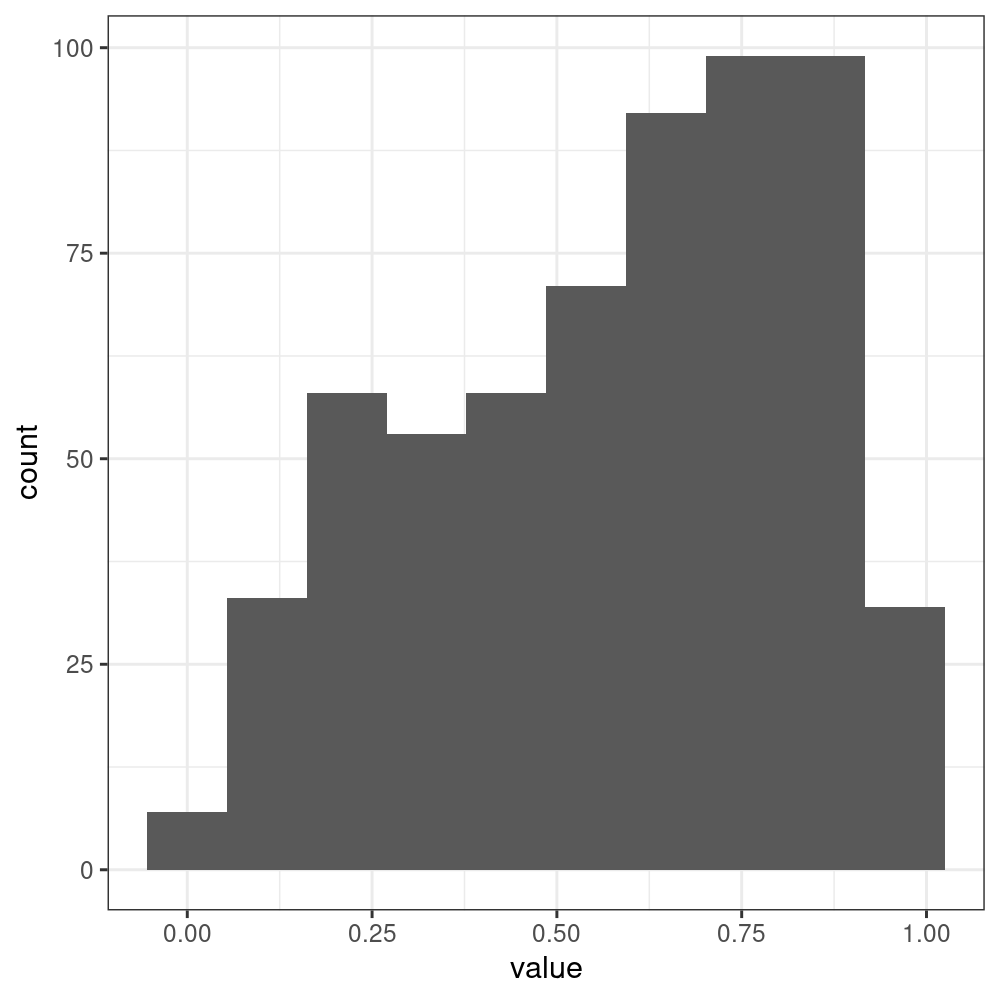
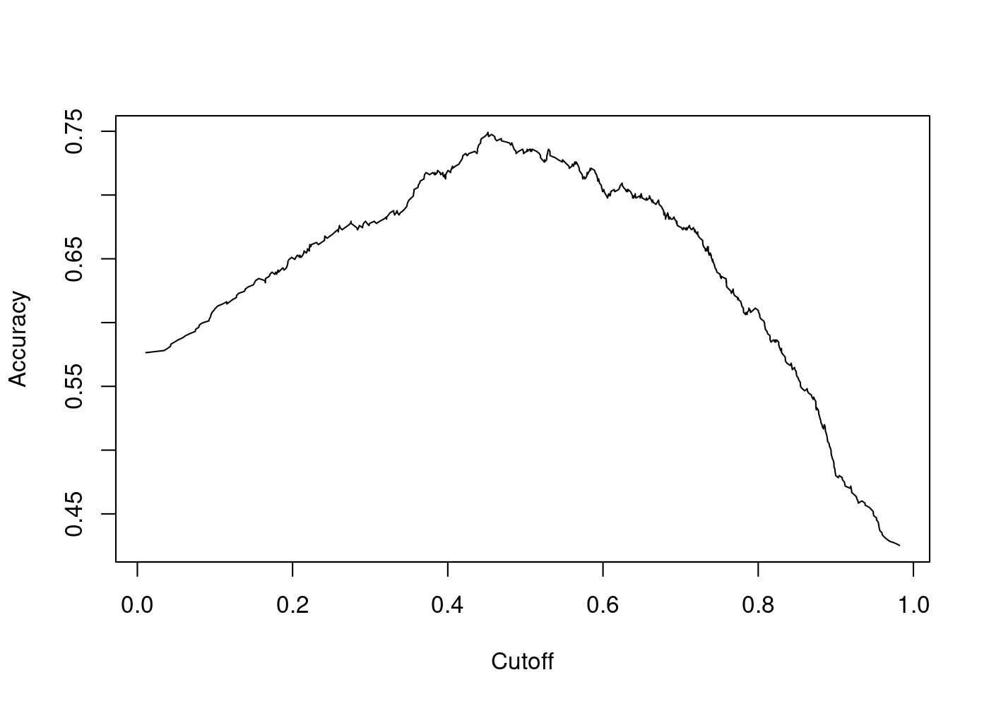
We can calculate the \(\widehat{\mathbb{P}}(Y = 1 | \mathbf{X})\) as follows: