# logistic regression:
rocr_pred_logit <- ROCR::prediction(predict(logit_glm, newdata = dt_train, type = "response"), dt_train$inlf)
dt_auroc_logit  <- ROCR::performance(rocr_pred_logit, "tpr", "fpr")
auc_logit       <- ROCR::performance(rocr_pred_logit, measure = "auc")@y.values[[1]]
# k-NN
rocr_pred_knn <- ROCR::prediction(predict(mdl_knn, newdata = dt_train, type = "prob")[, "1"], dt_train$inlf)
dt_auroc_knn  <- ROCR::performance(rocr_pred_knn, "tpr", "fpr")
auc_knn       <- ROCR::performance(rocr_pred_knn, measure = "auc")@y.values[[1]]
# Classification Tree:
rocr_pred_cdt <- ROCR::prediction(predict(mdl_cdt, newdata = dt_train, type = "prob")[, "1"], dt_train$inlf)
dt_auroc_cdt  <- ROCR::performance(rocr_pred_cdt, "tpr", "fpr")
auc_cdt       <- ROCR::performance(rocr_pred_cdt, measure = "auc")@y.values[[1]]
# LDA
rocr_pred_lda <- ROCR::prediction(predict(mdl_lda, newdata = dt_train, type = "prob")$posterior[, "1"], dt_train$inlf)
dt_auroc_lda  <- ROCR::performance(rocr_pred_lda, "tpr", "fpr")
auc_lda       <- ROCR::performance(rocr_pred_lda, measure = "auc")@y.values[[1]]
# QDA
rocr_pred_qda <- ROCR::prediction(predict(mdl_qda, newdata = dt_train, type = "prob")$posterior[, "1"], dt_train$inlf)
dt_auroc_qda  <- ROCR::performance(rocr_pred_qda, "tpr", "fpr")
auc_qda       <- ROCR::performance(rocr_pred_qda, measure = "auc")@y.values[[1]]
# NB
rocr_pred_nbc <- ROCR::prediction(predict(mdl_nbc, newdata = dt_train, type = "raw")[, "1"], dt_train$inlf)
dt_auroc_nbc  <- ROCR::performance(rocr_pred_nbc, "tpr", "fpr")
auc_nbc <- ROCR::performance(rocr_pred_nbc, measure = "auc")@y.values[[1]]Model comparison on the training set
Note
After estimating the different models, we now compare their results.
We begin by calculating the ROC curves:
11p <- data.table::rbindlist(list(
data.table(mdl = "Logistic regression", FPR = dt_auroc_logit@x.values[[1]], TPR = dt_auroc_logit@y.values[[1]]),
data.table(mdl = "k-NN", FPR = dt_auroc_knn@x.values[[1]], TPR = dt_auroc_knn@y.values[[1]]),
data.table(mdl = "Classification Tree", FPR = dt_auroc_cdt@x.values[[1]], TPR = dt_auroc_cdt@y.values[[1]]),
data.table(mdl = "LDA", FPR = dt_auroc_lda@x.values[[1]], TPR = dt_auroc_lda@y.values[[1]]),
data.table(mdl = "QDA", FPR = dt_auroc_qda@x.values[[1]], TPR = dt_auroc_qda@y.values[[1]]),
data.table(mdl = "Naive Bayes", FPR = dt_auroc_nbc@x.values[[1]], TPR = dt_auroc_nbc@y.values[[1]])
))11p_autoc <- p %>%
ggplot(aes(x = FPR, y = TPR)) +
geom_line(aes(color = mdl)) +
labs(x = dt_auroc_logit@x.name, y = dt_auroc_logit@y.name, title = "ROC Curve") +
theme_bw()
#
print(p_autoc)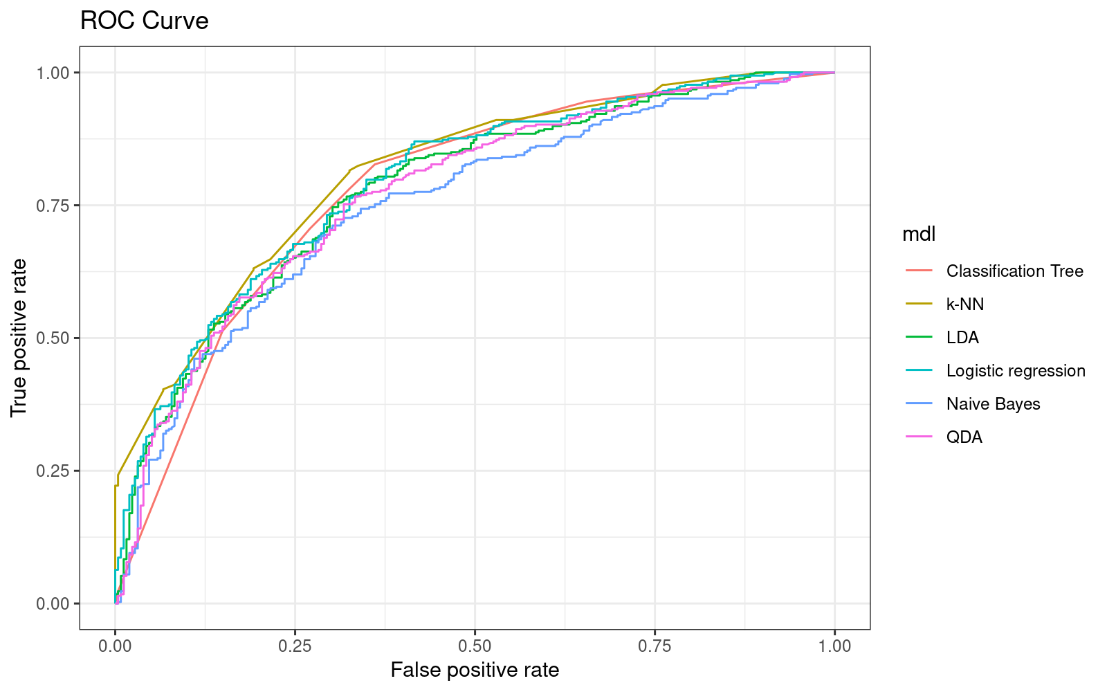
11data.table(mdl = c("Logistic regression", "k-NN", "Classification Tree", "LDA", "QDA", "Naive Bayes"),
AUC = c(auc_logit, auc_knn, auc_cdt, auc_lda, auc_qda, auc_nbc)) %>%
.[order(-AUC)] mdl AUC
1: k-NN 0.8098774
2: Logistic regression 0.7935469
3: LDA 0.7798384
4: Classification Tree 0.7793694
5: QDA 0.7723569
6: Naive Bayes 0.750545311In-sample, the best model was \(k\)-NN.
Note - we can calcualte the optimal cutoffs as follows:
# Logistic regression
opt_cutoff_logit <- ROCR::performance(rocr_pred_logit, measure = "acc")
opt_cutoff_logit <- opt_cutoff_logit@x.values[[1]][which.max(opt_cutoff_logit@y.values[[1]])]
# kNN
opt_cutoff_knn <- ROCR::performance(rocr_pred_knn, measure = "acc")
opt_cutoff_knn <- opt_cutoff_knn@x.values[[1]][which.max(opt_cutoff_knn@y.values[[1]])]
# Classification Tree
opt_cutoff_cdt <- ROCR::performance(rocr_pred_cdt, measure = "acc")
opt_cutoff_cdt <- opt_cutoff_cdt@x.values[[1]][which.max(opt_cutoff_cdt@y.values[[1]])]
# LDA
opt_cutoff_lda <- ROCR::performance(rocr_pred_lda, measure = "acc")
opt_cutoff_lda <- opt_cutoff_lda@x.values[[1]][which.max(opt_cutoff_lda@y.values[[1]])]
# QDA
opt_cutoff_qda <- ROCR::performance(rocr_pred_qda, measure = "acc")
opt_cutoff_qda <- opt_cutoff_qda@x.values[[1]][which.max(opt_cutoff_qda@y.values[[1]])]
# NB
opt_cutoff_nbc <- ROCR::performance(rocr_pred_nbc, measure = "acc")
opt_cutoff_nbc <- opt_cutoff_nbc@x.values[[1]][which.max(opt_cutoff_nbc@y.values[[1]])]11