Other Classification methods

Note

This section continues on from the end of the previous section on exploratory data analysis.

\(k\)-Nearest Neighbors

For the \(k\)-Nearest neighbors classification, we will only use continuous explanatory variables.

We shouldn’t forget to re-scale our data:

dt_train[, .(educ, educ_sc = c(scale(educ)), exper, exper_sc = c(scale(exper)), kidslt6, kidslt6_sc = c(scale(kidslt6)))]
     educ    educ_sc exper    exper_sc kidslt6 kidslt6_sc
  1:   14  0.7685500     1 -1.20320401       0 -0.4634363
  2:   12 -0.1194867    10 -0.07827574       2  3.3583263
  3:   12 -0.1194867     8 -0.32825980       0 -0.4634363
  4:   11 -0.5635050     3 -0.95321995       0 -0.4634363
  5:   13  0.3245317     4 -0.82822792       0 -0.4634363
 ---                                                     
598:   13  0.3245317    25  1.79660471       0 -0.4634363
599:   12 -0.1194867     9 -0.20326777       0 -0.4634363
600:   12 -0.1194867    11  0.04671629       1  1.4474450
601:   15  1.2125683    14  0.42169238       0 -0.4634363
602:   15  1.2125683    16  0.67167644       0 -0.4634363
1
1
Important

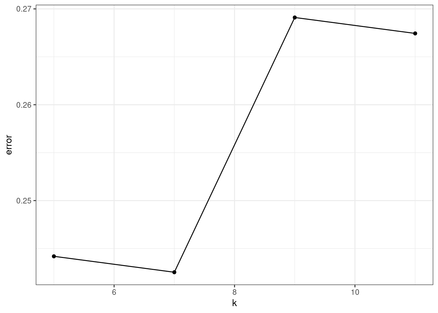
The value of \(k\) in the KNN algorithm is related to the error rate of the model. A small value of \(k\) could lead to overfitting, while a big value of \(k\) can lead to underfitting.

For binary data we want to avoid the case of ties. For example, if \(k = 2\), then we could have a case when one neighbor is \(Y = 0\) and the other one is \(Y = 1\).

Since we want to avoid overfitting - we will start from \(k = 5\).

misclasserror <- data.frame(k = c(5, 7, 9, 11), error = NA)
for(i in 1:nrow(misclasserror)){
  mdl_knn <- caret::knn3(factor(inlf) ~ scale(educ) + scale(exper) + scale(age) + scale(kidslt6) + scale(kidsge6), 
                         data = dt_train, k = misclasserror$k[i])
  dt_tst <- data.frame(actual = factor(dt_train$inlf),
                       predicted = predict(mdl_knn, dt_train, type = "class")) %>%
    as.data.table()
  misclasserror$error[i] <- 1 - dt_tst[, .(sum(actual == predicted) / .N)] %>% unlist()
}
1
1
misclasserror %>% ggplot(aes(x = k, y = error)) + 
  geom_line() + geom_point() + theme_bw()

1
1
Important

We have to be very carefull and include only explanatory variables, avoiding varibales like hours, wage, nwifeinc, etc., which have specific values as a consequence of being in the labor force.

optimal_k = misclasserror$k[misclasserror$error == min(misclasserror$error)]
print(optimal_k)
[1] 7
1
1

So, we fit our KNN algorithm with the optimal number of neighbors:

mdl_knn <- caret::knn3(factor(inlf) ~ scale(educ) + scale(exper) + scale(age) + scale(kidslt6) + scale(kidsge6), 
                         data = dt_train, k = optimal_k)
1
1

Which we can use to get the confusion matrix:

conf_mat_knn <- data.frame(actual = dt_train$inlf %>% as.character() %>% as.numeric(),
                      predicted = predict(mdl_knn, dt_train, type = "class") %>% as.character() %>% as.numeric()
                      )
conf_mat_knn <- table(conf_mat_knn)
conf_mat_knn
      predicted
actual   0   1
     0 170  85
     1  62 285
1
1
print(paste0("Misclassifications (k-NN): ", sum(sum(conf_mat_knn[lower.tri(conf_mat_knn) | upper.tri(conf_mat_knn)]))))
[1] "Misclassifications (k-NN): 147"
1
1
mdl_knn
7-nearest neighbor model
Training set outcome distribution:

  0   1 
255 347 
1
1

Classification (Decision) Trees

mdl_cdt <- rpart::rpart(factor(inlf) ~ educ + exper + age + kidslt6 + kidsge6, data = dt_train)
1
1
rpart.plot(mdl_cdt)

1
1

In a classification tree each node shows:

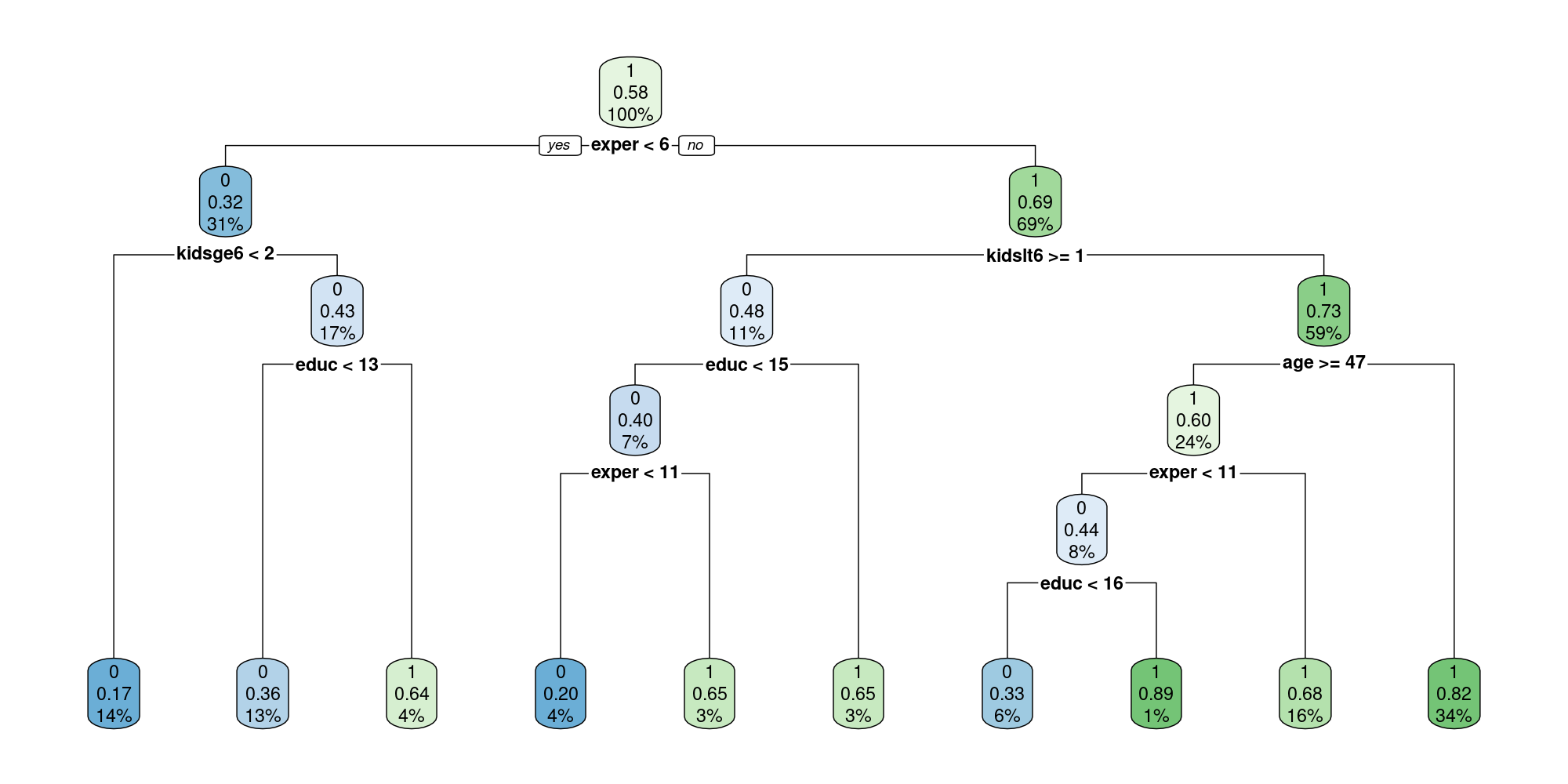
  • The predicted class (in our case - either 0 or 1).
  • The predicted probability
  • The percentage of observations in the node.

For example, at the first depth level - we see that if someone has less than 6 years of experience, then around \(31\%\) of (all) observations didn’t return to the labor force (the predicted probability is \(0.32\)), while \(69\%\) did return. Then, when we go one level down, we see that of those \(69\%\) who did return to the labor force, if they also had more than 1 child under 6 years old (kidslt6>=1), there is a probability of \(0.48\) that they won’t return to the labor force - around \(11\%\) of the total sample.

mdl_cdt
n= 602 

node), split, n, loss, yval, (yprob)
      * denotes terminal node

 1) root 602 255 1 (0.4235880 0.5764120)  
   2) exper< 5.5 184  58 0 (0.6847826 0.3152174)  
     4) kidsge6< 1.5 82  14 0 (0.8292683 0.1707317) *
     5) kidsge6>=1.5 102  44 0 (0.5686275 0.4313725)  
      10) educ< 12.5 77  28 0 (0.6363636 0.3636364) *
      11) educ>=12.5 25   9 1 (0.3600000 0.6400000) *
   3) exper>=5.5 418 129 1 (0.3086124 0.6913876)  
     6) kidslt6>=0.5 65  31 0 (0.5230769 0.4769231)  
      12) educ< 14.5 45  18 0 (0.6000000 0.4000000)  
        24) exper< 10.5 25   5 0 (0.8000000 0.2000000) *
        25) exper>=10.5 20   7 1 (0.3500000 0.6500000) *
      13) educ>=14.5 20   7 1 (0.3500000 0.6500000) *
     7) kidslt6< 0.5 353  95 1 (0.2691218 0.7308782)  
      14) age>=46.5 146  58 1 (0.3972603 0.6027397)  
        28) exper< 10.5 48  21 0 (0.5625000 0.4375000)  
          56) educ< 15.5 39  13 0 (0.6666667 0.3333333) *
          57) educ>=15.5 9   1 1 (0.1111111 0.8888889) *
        29) exper>=10.5 98  31 1 (0.3163265 0.6836735) *
      15) age< 46.5 207  37 1 (0.1787440 0.8212560) *
1
1

Naive Bayes, LDA and QDA

We fit the models as follows:

mdl_lda <- MASS::lda(factor(inlf) ~ educ + exper + age + kidslt6 + kidsge6, data = dt_train)
mdl_qda <- MASS::qda(factor(inlf) ~ educ + exper + age + kidslt6 + kidsge6, data = dt_train)
mdl_nbc <- e1071::naiveBayes(factor(inlf) ~ educ + exper + age + kidslt6 + kidsge6, data = dt_train)
1
1
mdl_lda
Call:
lda(factor(inlf) ~ educ + exper + age + kidslt6 + kidsge6, data = dt_train)

Prior probabilities of groups:
       0        1 
0.423588 0.576412 

Group means:
      educ     exper      age   kidslt6  kidsge6
0 11.77255  7.733333 42.97647 0.3764706 1.321569
1 12.63401 12.752161 41.65130 0.1440922 1.351585

Coefficients of linear discriminants:
                LD1
educ     0.18171773
exper    0.10324796
age     -0.08116898
kidslt6 -1.36933571
kidsge6  0.08923258
mdl_qda
Call:
qda(factor(inlf) ~ educ + exper + age + kidslt6 + kidsge6, data = dt_train)

Prior probabilities of groups:
       0        1 
0.423588 0.576412 

Group means:
      educ     exper      age   kidslt6  kidsge6
0 11.77255  7.733333 42.97647 0.3764706 1.321569
1 12.63401 12.752161 41.65130 0.1440922 1.351585
mdl_nbc

Naive Bayes Classifier for Discrete Predictors

Call:
naiveBayes.default(x = X, y = Y, laplace = laplace)

A-priori probabilities:
Y
       0        1 
0.423588 0.576412 

Conditional probabilities:
   educ
Y       [,1]     [,2]
  0 11.77255 2.117427
  1 12.63401 2.281186

   exper
Y        [,1]     [,2]
  0  7.733333 7.206151
  1 12.752161 7.896858

   age
Y       [,1]     [,2]
  0 42.97647 8.812540
  1 41.65130 7.585125

   kidslt6
Y        [,1]      [,2]
  0 0.3764706 0.6332606
  1 0.1440922 0.3979550

   kidsge6
Y       [,1]     [,2]
  0 1.321569 1.315611
  1 1.351585 1.284756
1
1