Model comparison on the test set

Note

After estimating the different models, we now compare their results.

We begin by calculating the ROC curves:

R
Python

# logistic regression:
rocr_pred_logit <- ROCR::prediction(predict(logit_glm, newdata = dt_test, type = "response"), dt_test$inlf)
dt_auroc_logit  <- ROCR::performance(rocr_pred_logit, "tpr", "fpr")
auc_logit       <- ROCR::performance(rocr_pred_logit, measure = "auc")@y.values[[1]]
# k-NN
rocr_pred_knn <- ROCR::prediction(predict(mdl_knn, newdata = dt_test, type = "prob")[, "1"], dt_test$inlf)
dt_auroc_knn  <- ROCR::performance(rocr_pred_knn, "tpr", "fpr")
auc_knn       <- ROCR::performance(rocr_pred_knn, measure = "auc")@y.values[[1]]
# Classification Tree:
rocr_pred_cdt <- ROCR::prediction(predict(mdl_cdt, newdata = dt_test, type = "prob")[, "1"], dt_test$inlf)
dt_auroc_cdt  <- ROCR::performance(rocr_pred_cdt, "tpr", "fpr")
auc_cdt       <- ROCR::performance(rocr_pred_cdt, measure = "auc")@y.values[[1]]
# LDA
rocr_pred_lda <- ROCR::prediction(predict(mdl_lda, newdata = dt_test, type = "prob")$posterior[, "1"], dt_test$inlf)
dt_auroc_lda  <- ROCR::performance(rocr_pred_lda, "tpr", "fpr")
auc_lda       <- ROCR::performance(rocr_pred_lda, measure = "auc")@y.values[[1]]
# QDA
rocr_pred_qda <- ROCR::prediction(predict(mdl_qda, newdata = dt_test, type = "prob")$posterior[, "1"], dt_test$inlf)
dt_auroc_qda  <- ROCR::performance(rocr_pred_qda, "tpr", "fpr")
auc_qda       <- ROCR::performance(rocr_pred_qda, measure = "auc")@y.values[[1]]
# NB
rocr_pred_nbc <- ROCR::prediction(predict(mdl_nbc, newdata = dt_test, type = "raw")[, "1"], dt_test$inlf)
dt_auroc_nbc  <- ROCR::performance(rocr_pred_nbc, "tpr", "fpr")
auc_nbc       <- ROCR::performance(rocr_pred_nbc, measure = "auc")@y.values[[1]]

R
Python

p <- data.table::rbindlist(list(
  data.table(mdl = "Logistic regression", FPR = dt_auroc_logit@x.values[[1]], TPR = dt_auroc_logit@y.values[[1]]),
  data.table(mdl = "k-NN", FPR = dt_auroc_knn@x.values[[1]], TPR = dt_auroc_knn@y.values[[1]]),
  data.table(mdl = "Classification Tree", FPR = dt_auroc_cdt@x.values[[1]], TPR = dt_auroc_cdt@y.values[[1]]),
  data.table(mdl = "LDA", FPR = dt_auroc_lda@x.values[[1]], TPR = dt_auroc_lda@y.values[[1]]),
  data.table(mdl = "QDA", FPR = dt_auroc_qda@x.values[[1]], TPR = dt_auroc_qda@y.values[[1]]),
  data.table(mdl = "Naive Bayes", FPR = dt_auroc_nbc@x.values[[1]], TPR = dt_auroc_nbc@y.values[[1]])
))

R
Python

p_autoc <- p %>%
  ggplot(aes(x = FPR, y = TPR)) + 
  geom_line(aes(color = mdl)) +
  labs(x = dt_auroc_logit@x.name, y = dt_auroc_logit@y.name, title = "ROC Curve") + 
  theme_bw()
#
print(p_autoc)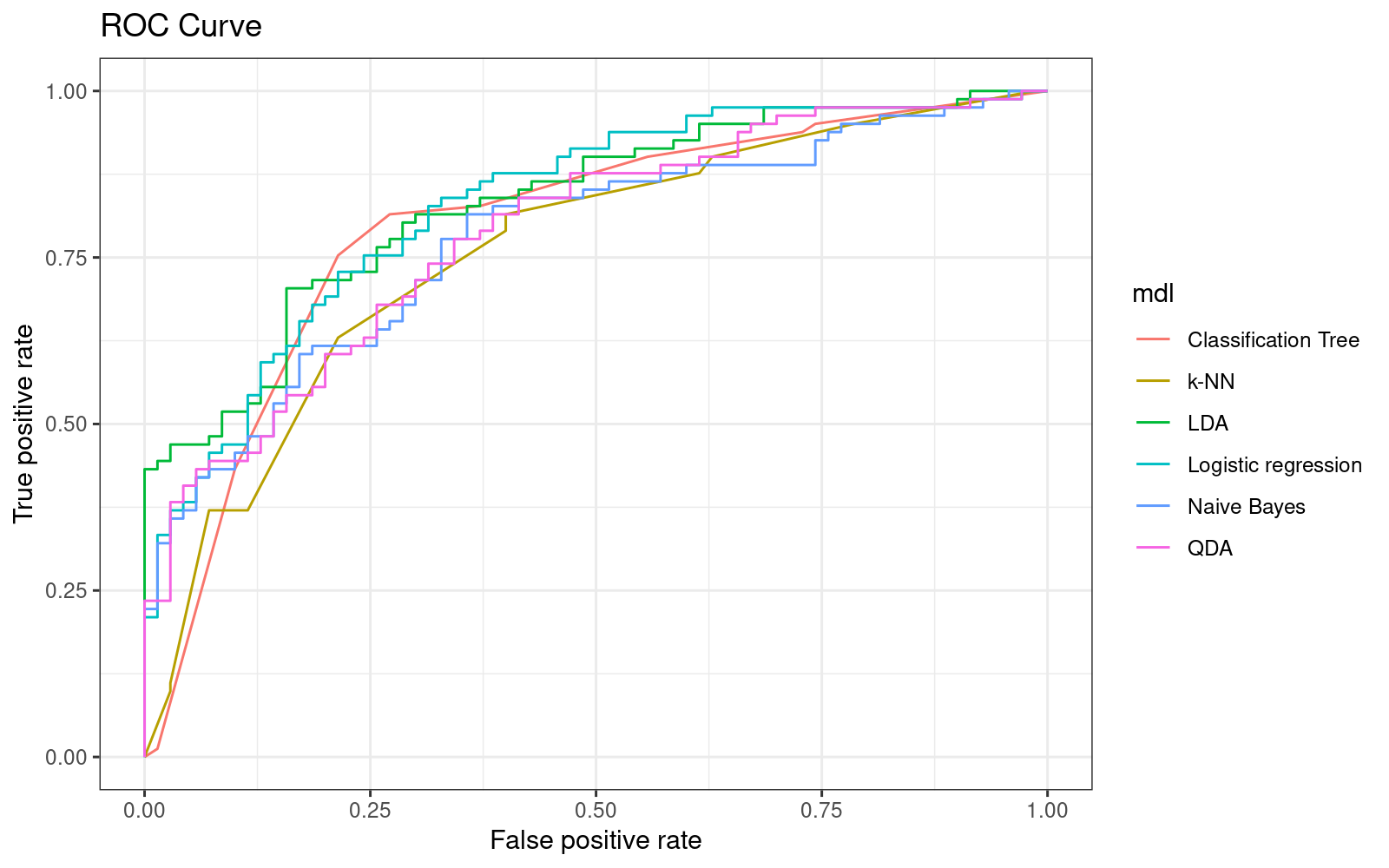

R
Python

data.table(mdl = c("Logistic regression", "k-NN", "Classification Tree", "LDA", "QDA", "Naive Bayes"),
           AUC = c(auc_logit, auc_knn, auc_cdt, auc_lda, auc_qda, auc_nbc)) %>%
  .[order(-AUC)]

                   mdl       AUC
1:                 LDA 0.8326279
2: Logistic regression 0.8291005
3: Classification Tree 0.7962081
4:                 QDA 0.7864198
5:         Naive Bayes 0.7776014
6:                k-NN 0.7582011

We can now make a number of conclusions:

\(k\)-NN, which was the best in-sample, now seems to perform the worst out-of-sample, suggesting that it fails to generalize to the broader data set.
logistic regression and LDA seem to perform equally great both in-sample and out-of-sample.
Logistic regression doesn’t make any assumptions about the distribution of the explanatory variables. As we-ve seen from the density charts - they don’t appear to be normally distributed. As a result, LDA may be a poor fit on this data.
Classification trees were similar in terms of their AUC to logistic regression, and their AUC changed only slightly in the test set.

Important

If we wanted to see how accurately our models predict a specific class, we can use the optimal cutoffs (required for the logistic regression), or simply choose to predict the class (valid for all models, except logistic regression).