Model adequacy

Note

This section continues on from the end of the previous section on prediction.

Visually comparing actual and fitted values

First, let’s visually compare the predicted (fitted) values against the actual ones.

predict_wage_train <- exp(predict(mdl_4, newdata = dt_train))
dt_compare <- cbind(actual = dt_train$wage, fitted = predict_wage_train) %>%
              as_tibble()
print(head(dt_compare, 10))
# A tibble: 10 × 2
   actual fitted
    <dbl>  <dbl>
 1   44.4   17.5
 2   16     19.5
 3   15.4   31.5
 4   13.5   21.0
 5   25     18.0
 6   24.0   24.6
 7   41.0   20.3
 8   26.4   27.7
 9   30.8   56.4
10   34.6   17.0
predict_wage_train = np.exp(mdl_4.predict(exog = dt_train))
dt_compare = pd.concat([dt_train["wage"], predict_wage_train], 
                        axis = 1, ignore_index = True).set_axis(labels = ['actual', 'fitted'], axis = 1)
print(dt_compare.head(10))
   actual     fitted
0   44.44  17.502749
1   16.00  19.539269
2   15.38  31.537529
3   13.54  20.965706
4   25.00  17.978159
5   24.05  24.588076
6   40.95  20.273622
7   26.45  27.681926
8   30.76  56.359195
9   34.57  16.963232

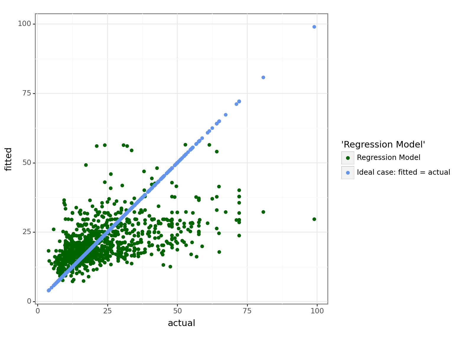
Ideally \(\widehat{Y} = Y\), however, remember that the the conditional expectation is the best predictor, which means that our predictions will have some degree of inaccuracy:

p1 <- dt_compare %>% 
  ggplot(aes(x = actual)) +
  geom_point(aes(y = fitted, color = "Regression Model")) + 
  geom_point(aes(y = actual, color = "Ideal case: fitted = actual")) +
  scale_color_manual(values = c("darkgreen", "cornflowerblue"),
                     name = element_blank()) +
  theme_bw()
print(p1)

p1 = (pl.ggplot(data = dt_compare, mapping = pl.aes(x = 'actual')) +\
  pl.geom_point(pl.aes(y = "fitted", color = "'Regression Model'")) + \
  pl.geom_point(pl.aes(y = "actual", color = "'Ideal case: fitted = actual'")) +\
  pl.scale_color_manual(values = ["darkgreen", "cornflowerblue"],
                     name = None) +\
  pl.theme_bw())
print(p1)

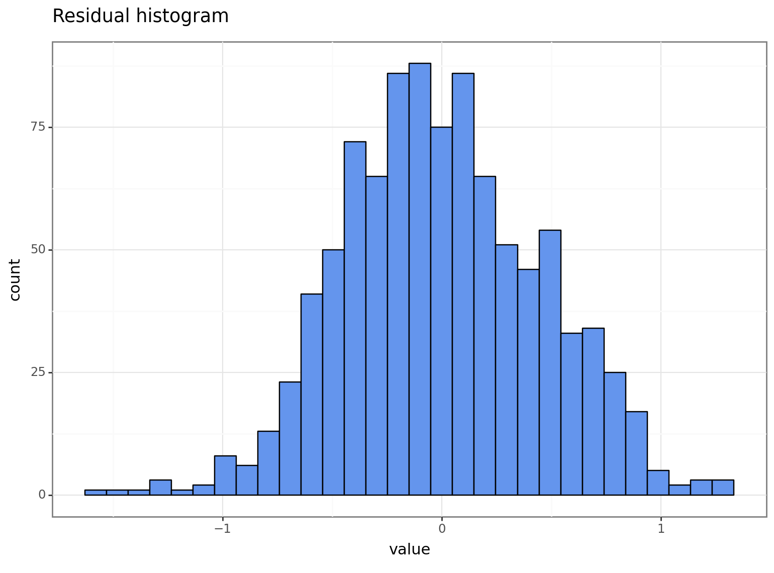
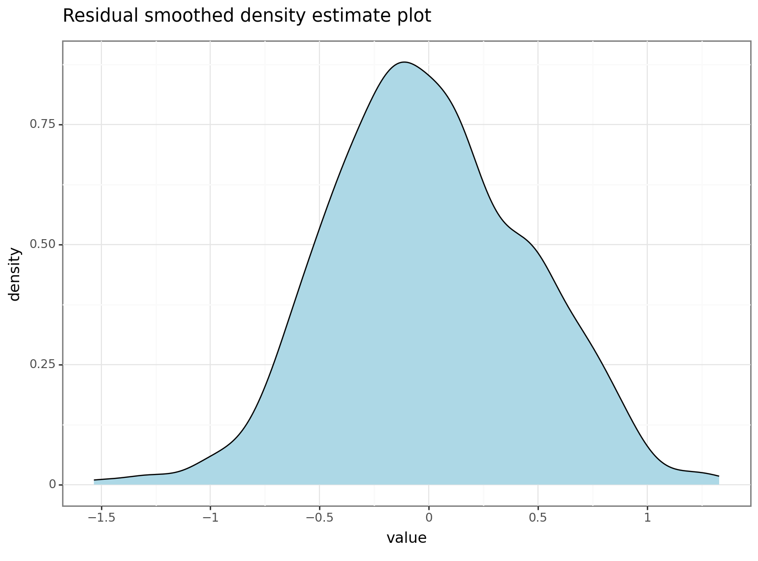
While plotting the “actual vs. fitted” values gives some insight, a more common approach is to analyse the model residuals. The residuals measure the difference between the actual and fitted values. As such, we will begin by visually examining their distribution:

p2 <- mdl_4 %>% residuals() %>% as_tibble() %>%
  ggplot(aes(x = value)) + 
  geom_histogram(bins = 30, color = "black", fill = "cornflowerblue") + 
  theme_bw() + labs(title = "Residual histogram")
p3 <- mdl_4 %>% residuals() %>% as_tibble() %>%
  ggplot(aes(x = value)) + 
  geom_density(fill = "lightblue") + 
  theme_bw() + labs(title = "Residual smoothed density estimate plot")
print(p2)
print(p3)

p2 = (pl.ggplot(data = pd.DataFrame(mdl_4.resid, columns = ["value"]), 
                mapping = pl.aes(x = 'value')) +\
  pl.geom_histogram(bins = 30, color = "black", fill = "cornflowerblue") +\
  pl.theme_bw() + pl.labs(title = "Residual histogram"))
p3 = (pl.ggplot(data = pd.DataFrame(mdl_4.resid, columns = ["value"]), 
                mapping = pl.aes(x = 'value')) +\
  pl.geom_density(fill = "lightblue") +\
  pl.theme_bw() + pl.labs(title = "Residual smoothed density estimate plot"))  
print(p2)
print(p3)

The residuals appear to visually be close to a normal distribution. Ideally, we would want our residual distribution to have a bell shape:

p4 <- mdl_4 %>% residuals() %>% as_tibble()
p4 <- p4 %>% ggplot() + 
  geom_density(aes(x = value, color = "Model residual distribution")) + 
  stat_function(aes(color = "Theoretical residual distribution"), 
                fun = dnorm, args = c(0, mdl_4 %>% sigma()), n = 1000, 
                xlim = c(min(mdl_4$residuals), max(mdl_4$residuals)), 
                show.legend = TRUE, linetype = "solid") + 
  theme_bw() + theme(legend.title = element_blank())
print(p4)

p4 = pd.DataFrame(mdl_4.resid, columns = ["value"])
p4 = (pl.ggplot(data = p4) +\
  pl.geom_density(pl.aes(x = "value", color = "'Model residual distribution'")) +\
  pl.stat_function(pl.aes(color = "'Theoretical residual distribution'"),\
                   fun = scipy.stats.norm.pdf, args = [0, np.sqrt(mdl_4.scale)], n = 1000, 
                   xlim = [min(mdl_4.resid), max(mdl_4.resid)], 
                   show_legend = True, linetype = "solid") +\
  pl.theme_bw() + pl.theme(legend_title = None))
print(p4)

Comparison with residuals from a simple regression

Notice that, compared to the residuals of a simple regression model for \(wage\) (instead of its logarithm) with one explanatory variable:

mdl_small_1 %>% residuals() %>% as_tibble() %>%
  ggplot(aes(x = value)) + geom_density(fill = "lightblue") + 
  theme_bw()

(pl.ggplot(data = pd.DataFrame(mdl_small_1.resid, columns = ["value"]),\
           mapping = pl.aes(x = "value")) + pl.geom_density(fill = "lightblue") +\
  pl.theme_bw())
<Figure Size: (770 x 570)>

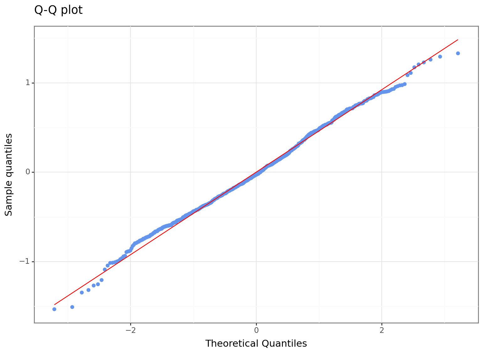
The residuals of our final model appear much closer (at least visually) to a normal distribution.

The above plot is only possible since we have a lot of observation to simulate the theoretical distribution. Another way to compare the actual residuals with the theoretical ones is by analysing their quantile-quantile plot:

p5 <- mdl_4 %>% residuals() %>% as_tibble() %>%
  ggplot(aes(sample = value)) + 
  stat_qq(color = "cornflowerblue") + stat_qq_line(color = "red") + 
  labs(title = "Q-Q plot") + 
  xlab("Theoretical Quantiles") + ylab("Sample quantiles") + 
  theme_bw()
print(p5)

p5 = (pl.ggplot(data = pd.DataFrame(mdl_4.resid, columns = ["value"]),\
                mapping = pl.aes(sample = "value")) +\
  pl.stat_qq(color = "cornflowerblue") + pl.stat_qq_line(color = "red") +\
  pl.labs(title = "Q-Q plot") + pl.xlab("Theoretical Quantiles") + pl.ylab("Sample quantiles") +\
  pl.theme_bw())
print(p5)

Here the red diagonal line is for the theoretical quantiles, while the blue dots are the quantiles of the model residuals.

While the graphical analysis gives us some insight, we cannot say for sure whether the residuals follow the theoretical assumptions from the Gauss-Markov theorem. We want to answer the following questions:

  • How close are our residuals to the normal distribution?
  • Are the residuals homoskedastic and do they exhibit autocorrelation?

To answer these questions, we will carry our a number of statistical tests.

Residual diagnostics tests

We will check for autocorrelation by testing the following hypothesis: \[ \begin{cases} H_0&:\text{the errors are serially uncorrelated (i.e. no autocorrelation)}\\ H_1&:\text{the errors are autocorrelated (the exact order of the autocorrelation depends on the test carried out)} \end{cases} \]

#
bg_test <- lmtest::bgtest(mdl_4, order = 3)
print(bg_test)

    Breusch-Godfrey test for serial correlation of order up to 3

data:  mdl_4
LM test = 2.9929, df = 3, p-value = 0.3927
name = ['LM statistic', 'LM p-value', 'F-value', 'F  p-value']
bg_test = sm.stats.acorr_breusch_godfrey(mdl_4, nlags = 3)
print(pd.DataFrame([np.round(bg_test, 8)], columns = name))
   LM statistic  LM p-value   F-value  F  p-value
0      2.992937    0.392715  0.990341    0.396594

The \(p-value = 0.3927 > 0.05\), so we have no grounds to reject the null hypothesis of no autocorrelation.

Which autocorrelation order should we choose?

We could test with higher order autocorrelation and examine the results by iterating through different autocorrelation orders:

for(i in 1:10){
      print(paste0("BG Test for autocorrelation order = ", i, 
                 "; p-value = ", round(lmtest::bgtest(mdl_4, order = i)$p.value, 2)))
}
[1] "BG Test for autocorrelation order = 1; p-value = 0.61"
[1] "BG Test for autocorrelation order = 2; p-value = 0.71"
[1] "BG Test for autocorrelation order = 3; p-value = 0.39"
[1] "BG Test for autocorrelation order = 4; p-value = 0.42"
[1] "BG Test for autocorrelation order = 5; p-value = 0.47"
[1] "BG Test for autocorrelation order = 6; p-value = 0.49"
[1] "BG Test for autocorrelation order = 7; p-value = 0.61"
[1] "BG Test for autocorrelation order = 8; p-value = 0.53"
[1] "BG Test for autocorrelation order = 9; p-value = 0.63"
[1] "BG Test for autocorrelation order = 10; p-value = 0.6"
for i in range(1, 11):
  tmp_val = sm.stats.acorr_breusch_godfrey(mdl_4, nlags = i)[1]
  print(f"BG Test for autocorrelation order = {i}; p-value = {round(tmp_val, 2)}")
BG Test for autocorrelation order = 1; p-value = 0.61
BG Test for autocorrelation order = 2; p-value = 0.71
BG Test for autocorrelation order = 3; p-value = 0.39
BG Test for autocorrelation order = 4; p-value = 0.42
BG Test for autocorrelation order = 5; p-value = 0.47
BG Test for autocorrelation order = 6; p-value = 0.49
BG Test for autocorrelation order = 7; p-value = 0.61
BG Test for autocorrelation order = 8; p-value = 0.53
BG Test for autocorrelation order = 9; p-value = 0.63
BG Test for autocorrelation order = 10; p-value = 0.6

As before - we see that there is no significant autocorrelation, as we have no grounds to reject the null hypothesis in all cases.

Note that carrying out multiple hypothesis tests leads to the multiple comparison problem. In reality, we would not try to re-do the same tests for different autocorrelation orders and instead select an order which would make sense (e.g., maybe the data is ordered by family members, so only \(2\) to \(4\) closest observations could be correlated).

We will now check for heteroskedasticity by carrying out a test for the following hypothesis: \[ \begin{cases} H_0&: \text{residuals are homoskedastic}\\ H_1&: \text{residuals are heteroskedastic} \end{cases} \]

#
bp_test <- lmtest::bptest(mdl_4)
print(bp_test)

    studentized Breusch-Pagan test

data:  mdl_4
BP = 27.891, df = 6, p-value = 9.851e-05
name = ['LM statistic', 'LM p-value', 'F-value', 'F  p-value']
bp_test = sm.stats.het_breuschpagan(resid = mdl_4.resid, exog_het = mdl_4_spec.exog)
print(pd.DataFrame([np.round(bp_test, 8)], columns = name))
   LM statistic  LM p-value   F-value  F  p-value
0     27.891003    0.000099  4.752686    0.000088

We have that the \(p\)-value \(< 0.05\), so we reject the null hypothesis that the residuals are homoskedastic. Which means that the residuals are heteroskedastic.

Finally, we check the residual normality by testing the following hypothesis:

\[ \begin{cases} H_0&:\text{residuals follow a normal distribution}\\ H_1&:\text{residuals do not follow a normal distribution} \end{cases} \] We will carry out a number of tests and combine their p-values into a single output:

norm_tests = c("Anderson-Darling", "Shapiro-Wilk", 
               "Kolmogorov-Smirnov (with specified parameters)", 
              "Cramer-von Mises", "Jarque-Bera")
norm_test <- data.frame(
    p_value = c(nortest::ad.test(mdl_4$residuals)$p.value,
                shapiro.test(mdl_4$residuals)$p.value,
                ks.test(mdl_4$residuals, y = "pnorm", 
                        0, sigma(mdl_4),  # (mean, sigma)
                        alternative = "two.sided")$p.value,
                nortest::cvm.test(mdl_4$residuals)$p.value,
                tseries::jarque.bera.test(mdl_4$residuals)$p.value),
    Test = norm_tests)
Warning in ks.test.default(mdl_4$residuals, y = "pnorm", 0, sigma(mdl_4), : ties should not be present for the Kolmogorov-Smirnov test
norm_tests = ["Anderson-Darling", "Shapiro-Wilk",  
              "Kolmogorov-Smirnov (with estimated parameters)", "Kolmogorov-Smirnov (with specified parameters)", 
              "Cramer-von Mises", "Jarque-Bera"]
norm_test = pd.DataFrame()
norm_test["p_value"] = [
    sm.stats.normal_ad(x = mdl_4.resid)[1],
    scipy.stats.shapiro(x = mdl_4.resid)[1],
    sm.stats.diagnostic.kstest_normal(x = mdl_4.resid, dist = "norm")[1],
    scipy.stats.kstest(rvs = mdl_4.resid, cdf = "norm", args = (0,np.sqrt(np.var(mdl_4.resid)))).pvalue,
    scipy.stats.cramervonmises(rvs = mdl_4.resid, 
                               cdf = "norm", 
                               args = (0, np.sqrt(np.var(mdl_4.resid))) # (mean, sigma)
                               ).pvalue,
    sm.stats.jarque_bera(mdl_4.resid)[1]
]
norm_test["Test"] = norm_tests              
print(norm_test)
      p_value                                           Test
1 0.002984346                               Anderson-Darling
2 0.014410937                                   Shapiro-Wilk
3 0.362223501 Kolmogorov-Smirnov (with specified parameters)
4 0.005107347                               Cramer-von Mises
5 0.739847087                                    Jarque-Bera
print(norm_test)           
    p_value                                            Test
0  0.002984                                Anderson-Darling
1  0.014411                                    Shapiro-Wilk
2  0.054206  Kolmogorov-Smirnov (with estimated parameters)
3  0.353017  Kolmogorov-Smirnov (with specified parameters)
4  0.263316                                Cramer-von Mises
5  0.739847                                     Jarque-Bera
Important

Note that in the above tests there are differences between the results from R and Python due to different implementations of the Kolmogorov-Smirnov and Cramer-von Mises tests. For example, in the scipy.stats.cramervonmises function, we pass the mean and standard deviation parameters, while in sm.stats.diagnostic.kstest_normal the mean and variance parameters are estimated.

Generally, the Shapiro–Wilk test has the best power for a given significance, though it is best to not rely on a single test result.

We see that the \(p\)-value is less than the \(5\%\) significance level for the Anderson-Darling and Shapiro-Wilk tests (and the Cramer-von Mises in R), which would lead us to reject the null hypothesis of normality. On the other hand the \(p\)-value is greater than \(0.05\) for Jarque-Bera and Kolmogorov-Smirnov tests, leading us to not reject the null hypothesis of normality.

Since Shapiro–Wilk test has the best power for a given significance, we will go with its result and reject the null hypothesis of normality.

Overall, our conclusions are as follows:

  • The model residuals are not serially correlated.
  • The model residuals are heteroskedastic.
  • The model residuals are non-normally distributed.

Correcting the standard errors of our model

So, our model residuals violate the homoskedasticity assumption, as well as the normality assumption.

Since our model residuals violate the homoskedasticity assumption - we can correct the standard errors using \(\rm HCE\) (Heteroskedasticity-Consistent standard Errors). This is known as the White correction - it will not change the \(\widehat{\beta}^{(OLS)}\), which are unbiased and ineffective, but it will correct \(\widehat{\mathbb{V}{\rm ar}}\left( \widehat{\boldsymbol{\beta}}_{OLS} \right)\).

While there are many different \(\rm HCE\) specifications, evaluating the empirical power of the four methods - \(\rm HC0\), \(\rm HC1\), \(\rm HC2\) and \(\rm HC3\) - suggested that \(\rm HC3\) is a superior estimate, regardless of the presence (or absence) of heteroskedasticity.

The corrected coefficient estimate variance covariance matrix is used to correct the standard errors (and \(p\)-values) of our coefficients:

mdl_4_corrected_se <- lmtest::coeftest(mdl_4, vcov. = sandwich::vcovHC(mdl_4, type = "HC3"))[, ]
print(round(mdl_4_corrected_se, 4))
            Estimate Std. Error t value Pr(>|t|)
(Intercept)   1.5556     0.1811  8.5882   0.0000
educ          0.0367     0.0248  1.4830   0.1384
I(educ^2)     0.0025     0.0009  2.6851   0.0074
exper         0.0276     0.0045  6.1939   0.0000
I(exper^2)   -0.0004     0.0001 -4.3629   0.0000
metro         0.1334     0.0370  3.6032   0.0003
female       -0.1592     0.0302 -5.2679   0.0000
print(mdl_4.get_robustcov_results(cov_type = "HC3").summary2().tables[1].round(4))
                     Coef.  Std.Err.       t   P>|t|  [0.025  0.975]
Intercept           1.5556    0.1811  8.5882  0.0000  1.2002  1.9111
educ                0.0367    0.0248  1.4830  0.1384 -0.0119  0.0853
np.power(educ, 2)   0.0025    0.0009  2.6851  0.0074  0.0007  0.0043
exper               0.0276    0.0045  6.1939  0.0000  0.0189  0.0364
np.power(exper, 2) -0.0004    0.0001 -4.3629  0.0000 -0.0006 -0.0002
metro               0.1334    0.0370  3.6032  0.0003  0.0607  0.2060
female             -0.1592    0.0302 -5.2679  0.0000 -0.2186 -0.0999

Although we have corrected for heteroskedasticity - coefficient significance conclusions remain the same as before. This could mean that the heteroskedasticity is not severe enough to affect our statistical test conclusions.

Correcting for autocorrelation

If our residuals are autocorrelated, or autocorrelated and heteroskedastic - we can use \(\rm HAC\) (Heteroskedasticity-and-Autocorrelation-Consistent standard Errors).

mdl_4_corrected_se_v2 <- lmtest::coeftest(mdl_4, vcov. = sandwich::NeweyWest(mdl_4, lag = 1, adjust = FALSE))[, ]
print(round(mdl_4_corrected_se_v2, 4))
            Estimate Std. Error t value Pr(>|t|)
(Intercept)   1.5556     0.1749  8.8959   0.0000
educ          0.0367     0.0234  1.5692   0.1169
I(educ^2)     0.0025     0.0009  2.8826   0.0040
exper         0.0276     0.0042  6.5516   0.0000
I(exper^2)   -0.0004     0.0001 -4.7656   0.0000
metro         0.1334     0.0349  3.8223   0.0001
female       -0.1592     0.0293 -5.4342   0.0000
print(mdl_4.get_robustcov_results(cov_type = "HAC", maxlags = 1, use_correction = False).summary2().tables[1].round(4))
                     Coef.  Std.Err.       t   P>|t|  [0.025  0.975]
Intercept           1.5556    0.1713  9.0791  0.0000  1.2194  1.8919
educ                0.0367    0.0232  1.5818  0.1140 -0.0088  0.0823
np.power(educ, 2)   0.0025    0.0009  2.8694  0.0042  0.0008  0.0042
exper               0.0276    0.0043  6.4250  0.0000  0.0192  0.0361
np.power(exper, 2) -0.0004    0.0001 -4.6035  0.0000 -0.0006 -0.0002
metro               0.1334    0.0357  3.7341  0.0002  0.0633  0.2035
female             -0.1592    0.0297 -5.3572  0.0000 -0.2176 -0.1009

Note that this procedure accounts for both autocorrelation and heteroskedasticity.

After testing the residuals of our final model and (if need be) correcting the standard errors, we might further ask ourselves whether:

  • Removing insignificant coefficients really improves our model?
  • How does our model compare with a simple regression model, where we included only one variable?

Coefficient of determination and information criterion(-s)

Important

When comparing models via \(\rm AIC\), \(\rm BIC\), \(R^2\) and \(R^2_{adj}\) it is important that the dependent variable has the same transformation is all of the models, that are being compared.

Note that the models have the following explanatory variables:

mdl_small_2 %>% coef() %>% names() %>% print()
[1] "(Intercept)" "educ"       
mdl_1 %>% coef() %>% names() %>% print()
[1] "(Intercept)"      "educ"             "exper"            "metro"            "geographysouth"   "geographywest"    "geographymidwest" "female"           "black"           
mdl_4 %>% coef() %>% names() %>% print()
[1] "(Intercept)" "educ"        "I(educ^2)"   "exper"       "I(exper^2)"  "metro"       "female"     
print(mdl_small_2.params.index.to_list())
['Intercept', 'educ']
print(mdl_1.params.index.to_list())
['Intercept', 'geography[T.south]', 'geography[T.west]', 'geography[T.midwest]', 'educ', 'exper', 'metro', 'female', 'black']
print(mdl_4.params.index.to_list())
['Intercept', 'educ', 'np.power(educ, 2)', 'exper', 'np.power(exper, 2)', 'metro', 'female']

In terms of information criterions and coefficient of determination:

out_1 <- data.frame(name = c("mdl_small_2", "mdl_1", "mdl_4"))
out_1[, "AIC"] <- c(stats::AIC(mdl_small_2), stats::AIC(mdl_1), stats::AIC(mdl_4))
out_1[, "BIC"] <- c(stats::BIC(mdl_small_2), stats::BIC(mdl_1), stats::BIC(mdl_4))
out_1[, "R_sq"]<- c(mdl_small_2 %>% summary() %>% .[["r.squared"]], mdl_1 %>% summary() %>% .[["r.squared"]], mdl_4 %>% summary() %>% .[["r.squared"]])
out_1[, "R_sq_adj"] <-  c(mdl_small_2 %>% summary() %>% .[["adj.r.squared"]], mdl_1 %>% summary() %>% .[["adj.r.squared"]], mdl_4 %>% summary() %>% .[["adj.r.squared"]])
out_1 = pd.DataFrame(["mdl_small_2", "mdl_1", "mdl_4"], columns = ["name"])
out_1["AIC"] = [mdl_small_2.aic, mdl_1.aic, mdl_4.aic]
out_1["BIC"] = [mdl_small_2.bic, mdl_1.bic, mdl_4.bic]
out_1["R_sq"]= [mdl_small_2.rsquared, mdl_1.rsquared, mdl_4.rsquared]
out_1["R_sq_adj"]= [mdl_small_2.rsquared_adj, mdl_1.rsquared_adj, mdl_4.rsquared_adj]
print(out_1)
         name      AIC      BIC      R_sq  R_sq_adj
1 mdl_small_2 1321.035 1335.636 0.2560084 0.2552318
2       mdl_1 1239.552 1288.222 0.3264458 0.3207797
3       mdl_4 1212.659 1251.594 0.3423183 0.3381776
print(out_1)
          name          AIC          BIC      R_sq  R_sq_adj
0  mdl_small_2  1319.035147  1328.769014  0.256008  0.255232
1        mdl_1  1237.552355  1281.354755  0.326446  0.320780
2        mdl_4  1210.658799  1244.727332  0.342318  0.338178
Important

Note that the differences in \(AIC/BIC\) values is due to disagreements on how many degress of freedom should be include in the information criterion formula.

We see that adding additional variables leads to a more accurate model:

  • While the simple regression model explains around \(25.6\%\) of the variation in \(\log(wage)\), adding more variables increases \(R^2\) to \(0.326\) (the new model explains \(32.6\%\) of the variation in \(\log(wage)\)). Accounting for the additional coefficients, the adjusted \(R\)-squared is \(0.32\).
  • Dropping insignificant variables and including polynomial terms improves the model even further - the explanatory variables in the final model explain \(34\%\) of the variation in \(\log(wage)\), while the adjusted \(R\)-squared is also larger and is equal to \(0.338\).

In terms of Information Criterions we see that both \(\rm AIC\) and \(\rm BIC\) are lower for our final model, which means that it better describes our data.

Important

Remember - we can compare \(R^2\) and \(AIC/BIC\) for models with the same dependent variable (and its transformation).

Having identified the in-sample adequacy of our model on the modelled (i.e. transformed) data. We now look at the in-sample and out-of-sample accuracy of our model on the original data.

In-sample vs. out-of-sample

While we have examined the accuracy in terms of \(\log(wage)\) models - how well does our final model describe \(wage\) itself? To check this, we can calculate \(R^2_{adj}\) for \(wage\).

In order to do this, we will need to calculate \(R^2_{adj}\) ourselves. To make it easier (and not repeat the same calculation steps every time) we will define a function:

r_sq_adj <- function(actual, fitted, k = 1){
    # k - number of parameters, excluding the intercept 
    RSS <- sum((actual - fitted)^2, na.rm = TRUE)
    TSS <- sum((actual - mean(actual, na.rm = TRUE))^2, na.rm = TRUE)
    return(1 - (RSS / (length(actual) - k - 1)) / (TSS / (length(actual) - 1)))
}
def r_sq_adj(actual, fitted, k = 1):
    # k - number of parameters, excluding the intercept
    RSS = np.sum((actual - fitted)**2)
    TSS = np.sum((actual - np.mean(actual))**2)
    return 1 - (RSS / (len(actual) - k - 1)) / (TSS / (len(actual) - 1))

We can verify that this function works, by comparing it with the built-in results:

mdl_4 %>% summary() %>% .[["adj.r.squared"]] %>% round(8) %>% print()
[1] 0.3381776
r_sq_adj(actual = log(dt_train$wage), 
         fitted = predict(mdl_4, newdata = dt_train), 
         k = length(mdl_4$coefficients) - 1) %>% round(8) %>% print()
[1] 0.3381776
print(round(mdl_4.rsquared_adj, 8))
0.33817763
r_sq_adj(actual = np.log(np.array(dt_train['wage'])),
         fitted = mdl_4.predict(exog = dt_train),
         k = len(mdl_4.params) - 1).round(8)
0.33817763

The in-sample and out-of-sample results for \(\log(wage)\) are very similar to each other:

tmp_dt <- c(
  r_sq_adj(actual = log(dt_train$wage), 
           fitted = predict(mdl_4, newdata = dt_train), 
           k = length(mdl_4$coefficients) - 1),
  r_sq_adj(actual = log(dt_test$wage), 
           fitted = predict(mdl_4, newdata = dt_test), 
           k = length(mdl_4$coefficients) - 1)
)
tmp_dt <- data.frame(smple = c("in-sample", "out-of-sampple"), R2_adj = tmp_dt)
print(tmp_dt)
           smple    R2_adj
1      in-sample 0.3381776
2 out-of-sampple 0.3548700
tmp_dt = [
  r_sq_adj(actual = np.log(np.array(dt_train['wage'])),
           fitted = mdl_4.predict(exog = dt_train),
           k = len(mdl_4.params) - 1),
  r_sq_adj(actual = np.log(np.array(dt_test['wage'])),
           fitted = mdl_4.predict(exog = dt_test),
           k = len(mdl_4.params) - 1)         
]
tmp_dt = pd.DataFrame({'smpl': ["in-sample", "out-of-sample"], 'R2_adj': tmp_dt})
print(tmp_dt)
            smpl    R2_adj
0      in-sample  0.338178
1  out-of-sample  0.354870

which indicates that the model itself has a similar accuracy on new data, as it does on the training data set.

We can also calculate the in-sample, as well as the out-of-sample results of the untransformed \(wage\):

tmp_dt <- c(
  r_sq_adj(actual = dt_train$wage, 
         fitted = exp(predict(mdl_4, newdata = dt_train)), 
         k = length(mdl_4$coefficients) - 1),
  r_sq_adj(actual = dt_test$wage, 
           fitted = exp(predict(mdl_4, newdata = dt_test)), 
           k = length(mdl_4$coefficients) - 1)
)
tmp_dt <- data.frame(smple = c("in-sample", "out-of-sampple"), R2_adj = tmp_dt)
print(tmp_dt)
           smple    R2_adj
1      in-sample 0.2521555
2 out-of-sampple 0.1728997
tmp_dt = [
  r_sq_adj(actual = np.array(dt_train['wage']),
           fitted = np.exp(mdl_4.predict(exog = dt_train)),
           k = len(mdl_4.params) - 1),
  r_sq_adj(actual = np.array(dt_test['wage']),
           fitted = np.exp(mdl_4.predict(exog = dt_test)),
           k = len(mdl_4.params) - 1)         
]
tmp_dt = pd.DataFrame({'smpl': ["in-sample", "out-of-sample"], 'R2_adj': tmp_dt})
print(tmp_dt)
            smpl    R2_adj
0      in-sample  0.252156
1  out-of-sample  0.172900

We see that the in-sample and out-of-sample \(R^2_{adj}\) is much lower for \(wage\) compared to the one for \(\log(wage)\). This is due to the fact that \(\log(wage)\) has a linear, while \(wage\) has an exponential relationship to the explanatory variables.

To compare model prediction accuracy, we will define \(\rm RMSE\) and \(\rm MAPE\) as separate functions:

calc_rmse <- function(actual, fitted){
    return(sqrt(mean((actual - fitted)^2)))
}
calc_mape <- function(actual, fitted){
    return(100 * mean(abs((actual - fitted) / actual)))
}
def calc_rmse(actual, fitted):
  return(np.sqrt(np.mean((actual - fitted)**2)))
#
def calc_mape(actual, fitted):
  return 100 * np.mean(np.abs((actual - fitted) / actual))

These functions will make it easier to re-calculate these measures on different cases:

predict_log_wage_train <- mdl_4 %>% predict(newdata = dt_train)
predict_log_wage_test  <- mdl_4 %>% predict(newdata = dt_test)
dt_out <- data.frame(name = c("In-sample", "Out-of-sample"))
dt_out[, "RMSE_log_wage"] <- c(
  calc_rmse(actual = log(dt_train$wage), fitted = predict_log_wage_train),
  calc_rmse(actual = log(dt_test$wage), fitted = predict_log_wage_test)
)
dt_out[, "MAPE_log_wage"] <- c(
  calc_mape(actual = log(dt_train$wage), fitted = predict_log_wage_train),
  calc_mape(actual = log(dt_test$wage), fitted = predict_log_wage_test)
)
dt_out[, "RMSE_wage"] <- c(
  calc_rmse(actual = dt_train$wage, fitted = exp(predict_log_wage_train)),
  calc_rmse(actual = dt_test$wage, fitted = exp(predict_log_wage_test))
)
dt_out[, "MAPE_wage"] <- c(
  calc_mape(actual = dt_train$wage, fitted = exp(predict_log_wage_train)),
  calc_mape(actual = dt_test$wage, fitted = exp(predict_log_wage_test))
)
print(dt_out)
           name RMSE_log_wage MAPE_log_wage RMSE_wage MAPE_wage
1     In-sample     0.4512748      12.60194  12.07094  38.37468
2 Out-of-sample     0.4631598      12.33094  17.30957  37.69263
predict_log_wage_train = mdl_4.predict(exog = dt_train)
predict_log_wage_test  = mdl_4.predict(exog = dt_test)
dt_out = pd.DataFrame(["In-sample", "Out-of-sample"], columns = ["name"])
dt_out["RMSE_log_wage"] = [
  calc_rmse(actual = np.log(np.array(dt_train["wage"])), fitted = np.array(predict_log_wage_train)),
  calc_rmse(actual = np.log(np.array(dt_test["wage"])), fitted = np.array(predict_log_wage_test))
]
dt_out["MAPE_log_wage"] = [
  calc_mape(actual = np.log(np.array(dt_train["wage"])), fitted = np.array(predict_log_wage_train)),
  calc_mape(actual = np.log(np.array(dt_test["wage"])), fitted = np.array(predict_log_wage_test))
]
dt_out["RMSE_wage"] = [
  calc_rmse(actual = np.array(dt_train["wage"]), fitted = np.exp(np.array(predict_log_wage_train))),
  calc_rmse(actual = np.array(dt_test["wage"]), fitted = np.exp(np.array(predict_log_wage_test)))
]
dt_out["MAPE_wage"] = [
  calc_mape(actual = np.array(dt_train["wage"]), fitted = np.exp(np.array(predict_log_wage_train))),
  calc_mape(actual = np.array(dt_test["wage"]), fitted = np.exp(np.array(predict_log_wage_test)))
]
print(dt_out)
            name  RMSE_log_wage  MAPE_log_wage  RMSE_wage  MAPE_wage
0      In-sample       0.451275      12.601943  12.070936  38.374683
1  Out-of-sample       0.463160      12.330935  17.309566  37.692627

While \(\rm RMSE\) is more sensitive to the scale of data, both measures show that our final model exhibits similar accuracy for both in-sample and out-of-sample data.

\(\rm MAPE\) expresses accuracy as a percentage of the error - in our dataset a \(\rm MAPE\) value of \(12\%\) for \(\log(wage)\) indicates that, on average, the forecast of \(\log (wage)\) is off by \(12\%\). This translates to \(\approx 38\%\) forecast inaccuracy for \(wage\).

Furthermore, we see that the in-sample and out-of-sample values are close (both \(\rm RMSE\) and \(\rm MAPE\)) and are a contrast to the adjusted \(R^2_{adj.}\) value. One explanations is that the \(R^2_{adj.}\) value compares the ratio of the errors of our model, against the errors from the process average. In case of non-linearity (or back-transformation of the dependent variable), the \(R^2_{adj.}\) might be a poor choice as a measure of model adequacy.