[This is a supplementary material to Section 6.1 of Chapter 6]
An application of the Kirchhoff effective conductance formula
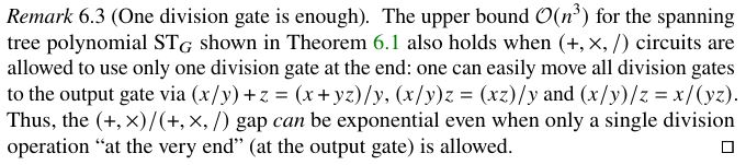
As shown in the book, unlike for non-monotone arithmetic $(+,\times,-)$ circuits (with subtraction), division $(/)$ gates (actually, only one division gate as the output gate, see Remark 6.3(1)) can even exponentially speed up monotone arithmetic $(+,\times)$ circuits.
The polynomial showing such a gap is defined using spanning trees of graphs.
Associate with each edge $e$ of $K_n$ a (formal)
variable $x_e$, interpreted as the weight of this edge. Let $G\subseteq K_n$ be a connected subgraph of the complete $n$ vertex graph $K_n$ on $[n]=\{1,\ldots,n\}$ (the graph $G$ being connected means that there is a path between any two its vertices).
A spanning tree of $G$ is its connected subgraph which has no cycles (is a tree) and includes all $n$ vertices of the graph $G$.
The Kirchhoff's polynomial (or the spanning tree polynomial) $\spol{G}$ of the graph $G$:
\begin{equation}\label{eq:tpol}
\spol{G}(x) = \sum_{T} \prod_{e\in T}x_e\,,
\end{equation}
where the sum is over all spanning trees of $G$.
For definiteness, if $n=1$ (just a single vertex), then we set $\spol{G}(x)=1$.
We already know that:
$\spol{K_n}$ requires monotone arithmetic $(+,\times)$ circuits of size $2^{\Omega(\sqrt{n})}$ (Theorem 3.16 in the book)
but
for every graph $G\subseteq K_n$ (including $G=K_n$), the polynomial $\spol{G}$ can be computed by a monotone arithmetic $(+,\times,/)$ circuit of size $O(n^3)$ (Theorem 6.1 in the book).
The upper bound $O(n^3)$ was proved by Fomin, Grigoriev, and Koshevoy
in [2], where they first show that a slightly weaker upper bound $O(n^4)$
follows fairly easily from two classical results established by electrical
engineers at least $100$ years ago: the Kirchhoff's effective conductance formula [1] and the machinery of star-mesh transformation. Here we will show how this happens.
For two vertices $a\neq b$ of a weighted $n$-vertex graph $G$, let
$G(a,b)$ denote the $(n-1)$-vertex graph obtained from $G$ by
gluing the vertex $a$ to vertex $b$ as follows:
glue together the vertices $a$ and $b$ into one vertex, then
remove the resulting loop (if any, i.e., if $\{a,b\}$ was
an edge of $G$), and for every vertex $u\not\in\{a,b\}$ which was adjacent to
both vertices $a$ and $b$, replace the old weight $x_{u,b}$ of the edge $\{u,b\}$ by
the new weight $x_{u,a}+x_{u,b}$.
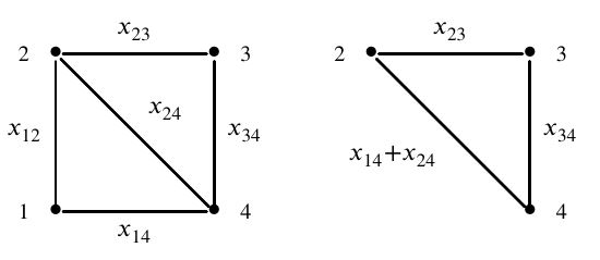
Fig. 1: A weighted graph $G$, and the graph $G(a,b)$ obtained by gluing vertex $a = 1$ to vertex $b=2$.
Interpret the weighted graph $G$ as an electric network with the
weight $x_e$ of each its edge $e$ interpreted as the electrical
conductance (the inverse $x_e=1/r_e$ of the electrical
resistance $r_e$) between the endpoints of $e$.
The Kirchhoff effective conductance formula [3] (see also [4], Section 2)
expresses the effective
conductance $\effcond{a,b}{G}$ between any two vertices $a$ and $b$ of
$G$ as the ratio of the Kirchhoff polynomial of the graph $G$ itself
and of the graph $G(a,b)$ obtained from $G$ by gluing vertex $a$
to vertex $b$.
Lemma A (Kirchhoff's effective conductance formula):
The effective conductance
between vertices $a$ and $b$ of $G$ is given by
\begin{equation}\label{eq:kirchhoff}
\effcond{a,b}{G} =\frac{\spol{G}}{\spol{G(a,b)}}\,.
\end{equation}
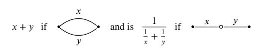
By Ohm's and Kirchhoff's laws, the conductance is additive for
resistors in parallel, and the resistance is additive for resistors in
series. That is, if we have two edges with conductances $x$ and $y$, then
the effective conductance between bold nodes is:
For example, due to the series-parallel property of the
particular graph $G$ in Fig 1, the effective conductance
between its vertices $1$ and $2$ can be computed as:
\[
\displaystyle \effcond{1,2}{G}=x_{12}+\displaystyle
\frac{1}{\displaystyle \frac{1}{x_{14}}+\frac{1}{x_{24}+\displaystyle
\frac{1}{x_{23}+x_{34}}}}\,.
\]
In general, not necessarily series-parallel graphs $G$, the
effective conductances between any two vertices can be recursively
computed using the well-known
machinery of star-mesh transformation developed by electrical
engineers at least $100$ years ago.
Take any vertex $u$ of $G$, and let $N(u)$ be the set
of all neighbors of $u$ in $G$.
Let $X_u:=\sum_{v\in N(u)}x_{uv}$ be the sum of weights of all
edges joining the vertex $u$ to its neighbors in $G$.
Remove the vertex $u$ together with all its incident edges.
For every $v\neq w\in N(u)$ draw and edge between $v$ and $w$
and give it weight
\[
x'_{vw}=\frac{x_{uv}\cdot x_{uw}}{X_u}\,.
\]
Replace parallel edges with one edge of accumulated weight. Hence,
if $\{v,w\}$ was an edge in $G$, then its new weight is
\[
x'_{vw}=x_{vw}+\frac{x_{uv}\cdot x_{uw}}{X_u}\,.
\]
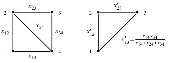
An example of this transformation is depicted in Fig 2.
Fig. 2: A graph $G$, and the graph obtained by applying the star-mesh transformation to the vertex $u=4$ of $G$.
New weights of the (old) edges $\{1,2\}$ and $\{2,3\}$ are:
\[
\displaystyle x'_{12}=x_{12}+\frac{x_{14}x_{24}}{x_{14}+x_{24}+x_{34}}\ \
\mbox{ and }\ \
x'_{23}=x_{23}+\frac{x_{24}x_{34}}{x_{14}+x_{24}+x_{34}}\,.
\]
It is long known (see, for example, [1, Corollary 4.21])) that
the effective conductance between any two vertices in the new weighted
graph $G'$ under the new weighting $x'$ is the same as the effective
conductance between these vertices in the old weighted graph $G$ under
the old weighting $x$.
Lemma B (Star-mesh transformation):
If $G'$ is the weighted graph obtained from $G$
by applying the star-mesh
transformation to a vertex $u$ of $G$, then for any two vertices $a$ and $b$
different from $u$, we have
\[
\effcond{a,b}{G'}=\effcond{a,b}{G}\,.
\]
Proof of the upper bound for (+,x,/) circuits
Take an arbitrary connected graph $G\subseteq K_n$. Our goal is to show that the polynomial $\spol{G}$ can be computed by a monotone arithmetic $(+,\times,/)$ circuit of size $O(n^4)$.
By treating the vertices $1,2,\ldots,n$ of $G$ one-by-one, we obtain
a sequence $G_1,\ldots,G_n$ of graphs, where $G_1=G$ and $G_{i+1}$
is a weighted graph on $\{i+1,\ldots,n\}$ obtained from $G_i$ by
gluing vertex $i$ to vertex $i+1$ in the graph $G_i$, that is,
$G_{i+1}=G_i(i,i+1)$.
For example, if $G$ is the graph in Fig 1, then $G_1=G$;
$G_2$ is the graph shown in Fig 1 (right); $G_3$ is a
two-vertex graph with a single edge of weight $x_{14}+x_{2
4}+x_{34}$; and $G_4$ (and more generally $G_n$) is a
single-vertex graph with no edges (so $\spol{G_n}=1$).
By Lemma A, we have
\[
\effcond{i,i+1}{G_i}= \frac{\spol{G_i}}{\spol{G_{i+1}}}\ \
\mbox{ for all }\ \ i=1,\ldots,n\,.
\]
So, the following formula is immediate via
telescoping:
\begin{equation}\label{eq:effcon-spantree}
\prod_{i=1}^{n-1}\effcond{i,i+1}{G_i}=\prod_{i=1}^{n-1}
\frac{\spol{G_i}}{\spol{G_{i+1}}}=\spol{G_1}=\spol{G}\,.
\end{equation}
Using the star-mesh transformations and Lemma B, effective conductance
$\effcond{i,i+1}{G}$ between the vertices $i$ and $i+1$ can be
computed by an arithmetic $(+,\times,/)$ circuit of size $O(n^3)$:
we have to recompute the weights for $O(n^2)$ pairs of vertices, and
for each pair $O(n)$ arithmetic $(+,\times,/)$ operations suffice.
So, the Kirchhoff polynomial
$\spol{G}$ can be computed by a $(+,\times,/)$ circuit of size
$O(n^4)$.
$\Box$
W. K. Chen: Graph theory and its engineering applications,
World Scientific, 1997.
S. Fomin and D. Grigoriev and G. Koshevoy: Subtraction-free complexity, cluster transformations, and spanning trees,
Found. Comput. Math.15 (2016) 1-31.
local copy
G. Kirchhoff: Über die Auflösung der Gleichungen, auf welche man bei der Untersuchungen der linearen Verteilung galvanischer Ströme geführt wird, Ann. Phys. Chem., 72 (1847) 497-508.
local copy
 Jump back ☝