Sets with large Sidon sets inside them are hard to produce

Also recall that a set $A\subseteq\NN^n$ is a Sidon set if the following holds for any vectors $a,b,c,d\in A$: \begin{equation}\label{eq:sidon} \text{if $a+b=c+d$ then $\{c,d\}=\{a,b\}$.} \end{equation} That is, if we know the sum of any two (not necessarily distinct) vectors of $A$, then we also know which vectors were added. Let us relax this condition and say that a subset $B\subseteq A$ of a set $A\subseteq\NN^n$ is a Sidon set inside $A$ if Eq. \eqref{eq:sidon} holds for all vectors $a,b\in B$ and $c,d\in A$.

Remark: Note that the mere fact that $B$ itself is a Sidon set is no longer sufficient: the sums $a+b$ of vectors in $B$ must now be unique not only within the set $B$ but also within the entire set $A$. Say, in the dimension $n=1$, $B=\{1,2,5,7\}$ is a Sidon set, but is not a Sidon set inside the set $A=\{1,2,4,5,7\}$ because $1+5=2+4$.

Theorem 2.18 in the book shows that $\Un{A}\geq |A|/2$ holds for every Sidon set $A\subseteq\NN^n$. Gashkov's [1] theorem (Theorem 2.6 in the book) gives a tighter lower bound $\Un{A}\geq |A|-1$ for such sets, which even holds for the number of union $(\cup)$ gates.

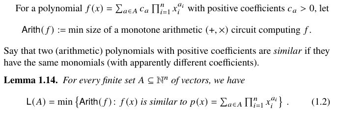
By Lemma 1.14⁽¹⁾, Gashkov's theorem implies that any monotone arithmetic $(+,\times)$ circuit computing a polynomial with positive coefficients, and whose set of exponent vectors is a Sidon set $A\subseteq\NN^n$, must use at least $|A|-1$ addition $(+)$ gates. Actually, Gashkov [1] stated and proved this lower bound for arithmetic $(+,\times)$ (not for Minkowski $(\cup,+)$) circuits, but since his argument only uses the structure of the sets $A$ of their exponent vectors, the bound holds also for Minkowski circuits.

A straightforward modification of the argument used in the proof of Theorem 2.18 in the book shows that a similar lower bound on $\Un{A}$ also holds for sets $A$ that themselves are not Sidon sets but contain sufficiently large subsets $B\subseteq A$ that are Sidon sets inside $A$.

Theorem A: Let $B\subseteq A\subseteq \NN^n$ and $|B|\geq 2$. If $B$ is a Sidon set inside $A$, then $\Un{A}\geq |B|/2$.

Proof (of Theorem A): Take a Minkowski $(\cup,+)$ circuit $\Phi$ which can use arbitrary singleton sets $\{x\}$ with $x\in\NN^n$ (not only the $n+1$ sets $\{\vec{0}\},\{\vec{e}_1\},\ldots,\{\vec{e}_n\}$) as inputs, and produces the set $A$. As in the book, we associate with every gate $v$ of $\Phi$ two sets $\pr{v}$ and $\compl{v}$ of vectors, where

• $\pr{v}\subseteq\NN^n$ is the set of vectors produced by the circuit $\Phi$ at gate $v$;
• $\compl{v}:=\{y\in\NN^n\colon \pr{v}+y\subseteq A\}$ is the set of all vectors $y\in\NN^n$ such that $x+y\in A$ holds for all vectors $x\in\pr{v}$.

Using our set $B\subseteq A$, we define subsets \[ \xpr{v}:=\{x\in \pr{v}\colon (x+\compl{v})\cap B\neq\emptyset\}\subseteq \pr{v}\ \ \mbox{ and }\ \ \xcompl{v}:=\{y\in \compl{v}\colon (\pr{v}+y)\cap B\neq\emptyset\}\subseteq \compl{v} \] of these two sets. That is, a vector $x\in\pr{v}$ belongs to $\xpr{v}$ if it can be extended to a vector of $B$ (not only of $A$) by adding some vector from $\compl{v}$, and similarly for vectors in $\xcompl{v}$.

To visualize the definition of sets $\xpr{v}$ and $\compl{v}$, associate with the set $A$ and with the gate $v$ bipartite graphs \[ G:=\{(x,y)\in \NN^{n\times n}\colon x+y\in A\}\qquad \mbox{and}\qquad G_v:=\{(x,y)\in \pr{v}\times\compl{v}\colon x+y\in B\}\,. \] Since $\pr{v}+\compl{v}\subseteq A$, the complete bipartite graph $\pr{v}\times \compl{v}$ is a subgraph of $G$. By their definition, the sets $\xpr{v}\subseteq \pr{v}$ and $\xcompl{v}\subseteq\compl{v}$ consist of all vertices of $G$ that are non-isolated in the subgraph $G_v$ of $G$.

Claim 1: For every gate $v$ of $\Phi$, we have $|\xpr{v}|\leq 1$ or $|\xcompl{v}|\leq 1$.

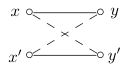
We clearly have $a+b=c+d$, but $x'\neq x$ and $y'\neq y$ yield $\{c,d\}\cap\{a,b\}=\emptyset$, meaning that $B$ is not a Sidon set inside $A$, a contradiction with the assumption of Theorem A. ∎

Recall that the content of a gate $v$ (of the circuit $\Phi$) is the rectangle $\econt{v}:=\pr{v}+\compl{v}$. Definition of contents of edges $e=(u,v)$ is asymmetric:

• $\econt{e}:=\pr{u}+\compl{v}$ if $v=u\cup w$ is a union gate;
• $\econt{e}:=\pr{v}+\compl{v}$ ($=\pr{u}+\pr{w}+\compl{v}=\econt{v}$) if $v=u+w$ is a Minkowski sum gate.

The reduced content $\xecont{e}$ of an edge is:

• $\xecont{e}:=\xpr{u}+\xcompl{v}\subseteq \econt{e}$ if $v=u\cup w$ is a union gate;
• $\xecont{e}:=\xpr{u}+\xpr{w}+\xcompl{v}\subseteq \econt{e}$ if $v=u+w$ is a Minkowski sum gate.

Claim 2 (Reduced contents): For every edge $e=(u,v)$ of the circuit $\Phi$, we have $\econt{e}\cap B\subseteq \xecont{e}$.

Proof: Let $e=(u,v)$ be an edge of the circuit $\Phi$, and let $w$ be the second gate entering the gate $v$. First suppose that $v=u\cup w$ is a union gate, and suppose that our vector $b\in B$ belongs to the content $\econt{e}=\pr{u}+\compl{v}$ of that edge $e$. Then $b=x+y$ for some $x\in \pr{u}\subseteq \pr{v}$ and $y\in \compl{v}\subseteq \compl{u}$. But then also $x\in\xpr{u}$ (since $y\in \compl{u}$) and $y\in\xcompl{v}$ (since $x\in\pr{v}$). Thus, the vector $b=x+y$ belongs to the reduced content $\xecont{e}=\xpr{u}+\xcompl{v}$ of the edge $e$, as desired.

Now suppose that $v=u+w$ is a Minkowski sum gate, and that our vector $b\in B$ belongs to the content $\econt{e}=\pr{v}+\compl{v}=\pr{u}+\pr{w}+\compl{v}$ of that edge $e$. Hence, $b=x_u+x_w+y$ for some vectors $x_u\in \pr{u}$, $x_w\in\pr{w}$ and $y\in \compl{v}$. Since $y\in\compl{v}$ and $\pr{v}=\pr{u}+\pr{w}$, we have $x_u+y\in\compl{w}$ and $x_w+y\in\compl{u}$ and, hence, also $x_u\in\xpr{u}$ and $x_w\in\xpr{w}$. Since clearly, $x_u+x_w\in \pr{v}$, we also have that $y\in\xcompl{v}$. Thus, the vector $b=x_u+x_w+y$ belongs to the reduced content $\xecont{e}=\xpr{u}+\xpr{w}+\xcompl{v}$ of the edge $e$, as desired. ∎

Claim 3 (Light edges): For every vector $b\in B$ there is an edge $e$ in the circuit $\Phi$ such that $\xecont{e}=\{b\}$.

Fix a vector $b\in B$. Start at the output gate of the circuit, and construct a path in the underlying directed acyclic graph by going backward and using the following rule, where $v$ is the last already reached gate.

1. If $v$ is a union $(\cup)$ gate, then follow an edge $e=(u,v)$ with $b\in \econt{e}$; if the vector $b$ belongs to contents of both edges entering $v$, then follow any one of these two edges.
2. If $v$ is a Minkowski sum $(+)$ gate, then go to either of the two inputs if they are both expensive or are both cheap and go to the expensive input if the second input is cheap.

Since our vector $b\in B$ belongs to the entire set $A$ produced by the circuit $\Phi$, the content propagation property (Lemma 2.19⁽²⁾) implies that the content of every edge along the entire path contains our vector $b$, and we will eventually reach some input gate. Since, by our assumption $|B|>1$, the output gate $v$ is expensive (because then $\pr{v}=A$ and $\compl{v}=\{\vec{0}\}$; hence, $\xpr{v}=B$). 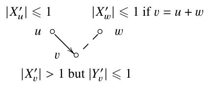Since each input gate is cheap, there must be an edge $e=(u,v)$ in this input-output path with the cheap tail $u$ and expensive head $v$, that is, with $|\xpr{u}|\leq 1$ and $|\xpr{v}|>1$. If $v=u+w$ is a Minkowski sum gate then, since the gate $u$ is cheap, step (2) in the construction of the path implies that the second gate $w$ entering $v$ must also be cheap, that is, $|\xpr{w}|\leq 1$ must hold as well. Moreover, $|\xpr{v}|>1$ and Claim 1 imply that $|\xcompl{v}|\leq l$ must hold for the gate $v$. Thus, we have the following information about our found edge $e=(u,v)$:

Since our vector $b\in B$ belongs to the content $\econt{e}$ of the found edge $e=(u,v)$, Claim 2 implies that $b$ also belongs to the reduced content $\xecont{e}$ of that edge. So, it remains to show that $|\xecont{e}|\leq 1$ (since $b\in\xecont{e}$, this will already yield the desired equality $\xecont{e}=\{b\}$).

If $v=u\cup w$ is a union gate, then $\xecont{e}=\pr{u}+\compl{v}$. Thus, $|\xecont{e}|=|\pr{u}+\compl{v}|\leq |\pr{u}|\cdot|\compl{v}|\leq 1$. If $v=u+w$ is a Minkowski sum gate, then the content of edge $e$ is the set $\xecont{e}=\xpr{u}+\xpr{w}+\xcompl{v}$. Since in this case, we additionally know that $|\xpr{w}|\leq 1$ holds for the second gate $w$, we have $|\xecont{e}|=|\xpr{u}|\cdot|\xpr{w}|\cdot|\xcompl{v}| \leq 1$. ∎

By Claim 3, for every vector $b\in B$ there is an edge $e$ of the circuit $\Phi$ whose content contains vector $b$ and no other vectors of $B$. Thus, the circuit must have at least $|B|$ edges and, hence, at least $|B|/2$ gates. This completes the proof of Theorem A. ∎

Remark: Theorem A properly extends Theorems 2.1 and 2.6 in the book because there are many non-Sidon sets with large Sidon sets inside them. To show this, let $S\subseteq\NN^n$ be any Sidon set, and be $T\subseteq\NN^n$ any set that is not a Sidon set. Assume for simplicity that neither $S$ nor $T$ contains the all-$0$ vector $\vec{0}$. Let $A=B\cup C$ be the union of two sets of vectors in $\NN^{2n}$, where $B$ consists of all vectors $(x,x)$ with $x\in S$, and $C$ consists of all vectors $(y,\vec{0})$ with $y\in T$. Then $B$ is a Sidon set because $S$ is such a set, but the entire set $A$ is not a Sidon set because already $T$ is not such a set. We claim that still, $B$ is a Sidon set inside $A$.

To show this, assume contrariwise that a sum $(x,x)+(z,z)$ of two vectors in $B$ is equal to a sum of some other two vectors in $A$. Since $B$ is a Sidon set, at least one of these two other vectors must belong to $C$, that is, must be of the form $(y,\vec{0})$ with $y\neq \vec{0}$. So we have $(x,x)+(z,z)=(y,\vec{0})+(u,v)$. If $(u,v)\not\in B$ then $v=\vec{0}$, and we obtain that $x+z=\vec{0}$, which is not possible because $x$ and $z$ are nonzero vectors. If $(u,v)\in B$ then $v=u$, and we obtain that $x+z=y+u$ and $x+z=\vec{0}+u$, which is also not possible because $y\neq \vec{0}$.    $\Box$

Footnotes:

^{(1)   Jump back ☝}

---

^{(2)   Jump back ☝}

---

References:

1. Gashkov, S.B.: On one method of obtaining lower bounds on the monotone complexity of polynomials. Vestnik MGU, Ser. 1 Math. Mech. 5, 7–13 (1987) . In Russian.   local copy

---

⇦   Back "Tropical Schnorr's bound"
or
⇦   Back to the comments page