Depth of tropical circuits

In the book, we were interested in the size of circuits. Another important measure is the circuit depth, that is, the maximum number of gates in an input-output path. If a circuit (over some semiring) has depth $d$, then its size $s$ satisfies $s\leq 2^d$ (gates have fanin $2$).

1. Upper Bounds

Theorem A ([6]): Let $A\subseteq\NN^n$ be a set of maximum degree $d$. If $A$ can be produced by a Minkowski circuit of size $s$, then $A$ can also be produced by a Minkowski circuit that has size $O(s^3)$ and depth $O((\log s)(\log d))$.

Example 1: Recall that the shortest $s$-$t$-path problem $\STPATH{n}$ is, given an assignment of nonnegative weights to the edges of the complete graph $K_n$ on the vertex-set $[n]=\{1,\ldots,n\}$, to compute the minimum weight of a simple path from vertex $s=1$ to vertex $t=n$, the latter being the sum of weights of edges of this path. Using binary search, one can easily construct a $(\min,+)$ circuit of depth $O(\log^2 n)$ for $\STPATH{n}$. But the size of the resulting circuit will then be $n^{\Omega(\log n)}$. To obtain a circuit of depth $O(\log^2 n)$ but polynomial size, we can take the $(\min,+)$ circuit $\Phi$ of size $O(n^3)$ resulting from the Bellman-Ford-Moore dynamic programming algorithm (see Example 1.8 in the book). Let $B\subseteq\NN^{\binom{n}{2}}$ be the set of vectors produced by the circuit $\Phi$. Every vector $b\in B$ (indexed by the edges of $K_n$) corresponds to an $s$-$t$ walk in $K_n$ with $\leq n-1$ edges, and $b_{i,j}$ being the number of times the edge $\{i,j\}$ appears in the walk $w_b$. Since the maximum degree of $B$ does not exceed $n-1$, Theorem A implies that the set $B$ can also be produced by a $(\min,+)$ circuit $\Phi'$ which simultaneously has depth $O(\log^2 n)$ and size $O(n^9)$. Since the new circuit $\Phi'$ produces the same set $B$, it also solves the problem $\STPATH{n}$.    $\Box$

To apply Theorem A to $(\min,+)$ circuits, we must know the maximum degrees of sets $B\subseteq \NN^n$ of vectors produced by them. In the case of $(\max,+)$ circuits, the situation is simpler: then the degree of any produced set $B$ cannot exceed the degree of the set of feasible solutions of a given maximization problem.

Corollary A: Let $A\subseteq\{0,1\}^n$ be an antichain. If the maximization problem on $A$ can be solved by a tropical $(\max,+)$ circuit of size $s$, then this problem can also be solved by a tropical $(\max,+)$ circuit of size $O(s^3)$ and depth $O((\log s)(\log n))$.

Remark A: Note that, in general, the argument used in the proof of Corollary A cannot give any reasonable upper bound for $(\min,+)$ circuits: unlike for $(\max,+)$ circuits, the sets $B\subseteq\NN^n$ of vectors produced by such circuits of size $s$ may have maximum degree up to $2^s$ (by Lemma 1.22, the set then $B$ lies above (not below) the set $A$. In Example 1, however, we already knew that the maximum degree of the set of vectors produced by a particular $(\min,+)$ circuit is at most $n-1$.    $\Box$

2. Lower Bounds

Example 2: Consider the shortest $s$-$t$ path problem $\STPATH{n}$ from Example 1 above. The Boolean version of this problem is the Boolean function $\STCONN{n}(x)$: decide whether there is a path between $s$ and $t$ in a given subgraph $G_x$ of $K_n$ specified by a Boolean input vector $x\in\{0 ,1\}^{\binom{n}{2}}$ (an edge $e$ of $K_n$ is present in the graph $G_x$ iff $x_e=1$). Karchmer and Wigderson [3]f used communication complexity arguments to show that every monotone Boolean circuit computing $\STCONN{n}$ must have depth at least $\Omega(\log^2n)$. Thus, by the ``Boolean bound'' (Lemma 1.30⁽¹⁾), every $(\min,+)$ circuit solving the problem $\STPATH{n}$ must have depth at least $\Omega(\log^2 n)$. This, in particular, implies that the depth of the $(\min,+)$ circuit of size $O(n^9)$ for $\STPATH{n}$, which we described in Example 1 above, is optimal.    $\Box$

Unfortunately, the task of proving nontrivial lower bounds on the depth and/or size of Boolean circuits is a rather nontrivial task and, for this reason, even for monotone circuits, only several such bounds are known so far.

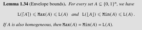
Fortunately, the task of proving lower bounds on the depth of Minkowski circuits (a.k.a. monotone arithmetic circuits) is easier. When this is done for Minkowski circuits producing homogeneous sets $A\subseteq\{0,1\}^n$ of vectors, then by Lemma 1.34⁽²⁾, the bound also holds for both optimization problems (minimization and maximization) on $A$.

Remark B: Although we stated and proved Lemma 1.34 in the book only for circuit size, it holds also for the circuit depth: when producing the lower and higher envelopes in Lemma 1.32⁽³⁾, we have not increased the circuit depth (we only removed some edges).    $\Box$

By simplifying the previous argument of Shamir and Snir [4], Tiwari and Tompa [5] have invented (on two examples) an interesting argument to prove lower bounds on the depth of monotone arithmetic circuits. Jukna [6] observed that the idea of Tiwari and Tompa fits into the following general frame (expressed by Lemmas A and B below).

2.1 General lower bound

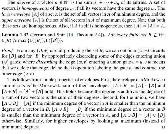
Now let $A\subseteq\NN^n$ be the set of vectors produced by the circuit $\Phi$, and suppose that this set is homogeneous of degree $m$ (all vectors $a\in A$ have the same degree $a_1+\cdots+a_n=m$). Since the produced set $A$ is homogeneous, the sets $\pr{v}\subseteq\NN^n$ of vectors produced at each gate $v$ of $\Phi$ must be homogeneous and, hence, all vectors of $\pr{v}$ have the same degree, which we denote by $\dg{v}$ and call the degree of the gate $v$.

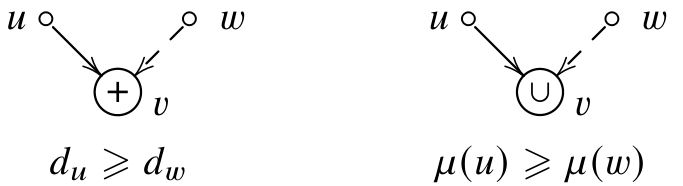
We call an input-to-output path $\pi$ in $\Phi$ balanced if every its edge $(u,v)$ has the following property, where $w$ is the second gate entering the gate $v$: if $v=u\cup w$ is a union gate, then $\dg{u}=\dg{w}=\dg{v}$, and if $v=u+w$ is a Minkowski sum gate, then $\dg{u}\geq \dg{w}$.

Lemma A: For every subadditive weighting $\wweight$ of the gates of $\Phi$, there is a balanced input-to-output path in $\Phi$ containing a sequence $v_1,\ldots,v_l$ of $l\geq \log_2m$ Minkowski sum $(+)$ gates and $p\geq \log_2 \prod_{i=1}^{l} \factor{v_i}$ union $(\cup)$ gates.

Construct an input-to-input path $\pi$ in a reversed order by going backward from the output gate (the last gate of the path $\pi$) to an input gate and using the following rule:

• at a Minkowski sum $(+)$ gate $v$ choose an input $u$ of greater degree;
• at a union $(\cup)$ gate $v$ choose the input $u$ of greater weight.

Now look at the path $\pi$ in a "normal" way as an input-to-output path. The path $\pi$ starts with some input gate (of weight $\leq 1$). Since the weighting is subadditive at union $(\cup)$ gates, at each edge entering a union gate the weight can only increase by a factor of at most $2$. So, if $p$ is the number of union gates along $\pi$, then the total increase in weight is by a factor at most $2^p$. But by Eq. \eqref{eq:decrease}, when entering the $i$th Minkowski sum $(+)$ gate $v_i$ along $\pi$, the weight decreases by a factor at least $1/\factor{v_i}$. Thus, the total decrease in the weight is by a factor at least $1/\prod_{i=1}^{l} \factor{v_i}$. Since the last (output) gate must have weight $\geq 1$, this gives \[ 2^p\cdot \prod_{i=1}^{l} \frac{1}{\factor{v_i}}\geq 1\,. \] Thus, the path $\pi$ must have $p\geq \log_2 \prod_{i=1}^{l} \factor{v_i}$ union gates, as desired. ∎

2.1 Specific lower bound

Lemma B: Let $A\subseteq \{0,1\}^n$ be a homogeneous set of degree $m$. Then there is a sequence $1=r_0 \lt r_1 \lt r_2 \lt \ldots \lt r_l=m$ of $l+1\geq \log_2 m$ integers such that $r_{i-1}\geq \frac{1}{2} r_{i}$ for all $i=0,1,\ldots,l$, and \[ \depth{A}\geq l+\log_2\prod_{i=1}^{l-1}\Factor{A}{r_i,r_{i-1}}\,. \]

Proof: Let $\Phi$ be a Minkowski $(\cup,+)$ circuit producing the set $A$, and $v$ be some its gate. Since the rectangle $\pr{v}+\compl{v}$ (the content of the gate $v$) lies in $A$, and since all vectors of $A$ have degree $m$, there must be a vector $y\in\compl{v}$ of degree at least $m-d_v$ for which $\pr{v}+y\subseteq A$ holds. So, since all vectors of $\pr{v}+y$ contain the vector $y$, we have $|\pr{v}|=|\pr{v}+y|\leq \Ddeg{A}{d_v}$. This suggests the following weighting of gates: \[ \weight{v}:=\frac{|\pr{v}|}{\Ddeg{A}{d_v}}\,. \] Intuitively, $\Ddeg{A}{d_v}$ is the maximal possible number of vectors that ``could'' be produced at the gate $v$ (so that the inclusion $\pr{v}+\compl{v}\subseteq A$ still holds), while $|\pr{v}|$ is the number of vectors produced at the gate $v$. For the output gate $o$, we have $\pr{o}=A$ and $d_o=m$. So, the output gate $o$ gets weight $\weight{o}=|A|/\Ddeg{A}{d_o} = |A|/\Ddeg{A}{m}= |A|/|A| =1$, whereas all other gates get weights $\leq 1$.

To apply Lemma A, we have to verify that our weighting is subadditive at union gates. To show this, let $v=u\cup w$ be a union gate; hence, $d_u=d_w=d_v$. So, since $|\pr{v}|=|\pr{u}\cup\pr{w}|\leq |\pr{u}|+|\pr{w}|$, the desired inequality $\weight{v}\leq \weight{u}+\weight{w}$ follows: \[ \weight{v}=\frac{|\pr{u}\cup\pr{w}|}{\Ddeg{A}{d_v}} \leq \frac{|\pr{u}|}{\Ddeg{A}{d_u}} +\frac{|\pr{w}|}{\Ddeg{A}{d_w}} =\weight{u}+\weight{w}\,. 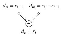\] Thus, our weighting is subadditive at union $(\cup)$ gates, as required. Let $\pi$ be a balanced input-to-output path in the circuit $\Phi$ guaranteed by Lemma A, and let $r_i$ be the degree $d_v$ of the $i$th of Minkowski sum $(+)$ gate $v$ along this path. Since the path $\pi$ is balanced, we have $d_u\geq d_w$ and, hence, also $d_u=r_{i-1}\geq \tfrac{1}{2}r_i$:

It remains to show that the decrease $\factor{v}$ of every Minkowski sum $(+)$ gate $v=u+w$ is at least $\Factor{A}{r_i,r_{i-1}}$. In fact, since $|\pr{v}|=|\pr{u}+\pr{w}|=|\pr{u}|\cdot|\pr{w}|$ and $d_w=d_v-d_u=r_i-r_{i-1}$, the decrease $\factor{v}$ of our weighting at the gate $v$ is exactly $\Factor{A}{r_i,r_{i-1}}$: \[ \factor{v}=\frac{\weight{u}\cdot \weight{w}}{\weight{v}} =\frac{\Ddeg{A}{d_{v}}}{|\pr{v}|}\cdot \frac{|\pr{u}|}{\Ddeg{A}{d_u}} \cdot \frac{|\pr{w}|}{\Ddeg{A}{d_w}}=\Factor{A}{r_i,r_{i-1}}. \tag*{$\Box$} \]

2.3 Applications

Corollary B: Let $A\subseteq\{0,1\}^{n\times n}$ be the set of all $|A|=n!$ characteristic vectors of perfect matchings in $K_{n,n}$. Then $\depth{A}\geq n + \log_2n -1$.

Note that a slightly weaker lower bound $\depth{A}=\Omega(n)$ for this set $A$ also follows from the lower bound $\Un{A}=2^{\Omega(n)}$ on the circuit size (Theorem 3.6 in the book), because we always have $\depth{A}\geq \log_2\Un{A}$. More interesting, however, is that Lemma B allows us to prove super-logarithmic depth lower bounds even for sets that have Minkowski circuits of polynomial size.

To demonstrate this, consider the iterated matrix multiplication polynomial. Let $X_1, X_2,\ldots, X_d$ be $d$ $n\times n$ matrices of indeterminates. Let $x_{i,j}^{(k)}$ denote the $(i,j)$-th entry of $X_k$. Let $P$ be the $(1,1)$-th entry of the product $X_1X_2\cdots X_d$ of these matrices. Hence, $P$ is the following homogeneous multilinear polynomial of degree $d$ with $(d-2)n^2+2n=\Theta(dn^2)$ variables: \[ P=\sum_{1\leq i_1,\ldots,i_{d-1}\leq n} x_{1,i_1}^{(1)}x_{i_1,i_2}^{(2)}x_{i_2,i_3}^{(3)}\cdots x_{i_{d-1},1}^{(d)}\,. \] It is convenient to view the monomials of $P$ as paths in the following layered graph $G=(V,E)$. We have $d+1$ layers $V_0,V_1,\ldots,V_d$ of nodes, where the first layer $V_0$ and the last layer $V_d$ consists of one node $1$, while each other layer consists of $n$ nodes $1,2,\ldots,n$. Edges of $G$ connect every node from one layer with all nodes of the next layer. Each edge $e=\{i,j\}\in V_{k-1}\times V_{k}$ of $G$ has its associated variable $x_{i,j}^{(k)}$, and the monomials $x_{1,i_1}^{(1)}x_{i_1,i_2}^{(2)}x_{i_2,i_3}^{(3)}\cdots x_{i_{d-1},1}^{(d)}$ of the polynomial $P$ correspond to the $n^{d-1}$ paths of length $d$ from the first to the last layer of $G$.

The monotone arithmetic circuit for the polynomial $P$ constructed according to the layered graph $G$ has size $O(dn^2)$ (linear in the number of variables of the polynomial $P$). Also, the product of two $n\times n$ matrices can be computed by a monotone arithmetic circuit of depth $O(\log n)$. Hence, by squaring, the polynomial $P$ can be computed by a monotone arithmetic circuit of depth $O((\log d)(\log n))$. The following corollary shows that the depth cannot be substantially reduced. Let $A\subseteq\{0,1\}^m$ be the set of $|A|=n^{d-1}$ exponent vectors of the monomials of $P$.

Corollary C: $\depth{A}=\Omega((\log d)(\log n))$.

^{(1)   Jump back ☝}

(2)   Jump back ☝

(3)   Jump back ☝