Contents
By Theorem 6.11(1), reciprocal inputs $-x_1,\ldots,-x_n$ (in addition to input variables $x_1,\ldots,x_n$) cannot substantially decrease
the size of tropical $(\min,+)$ circuits.
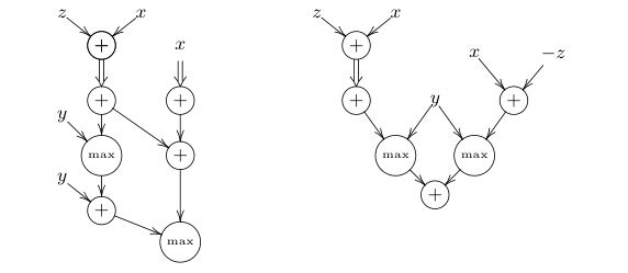
The situation with tropical $(\max,+,-x_i)$ circuits (solving
maximization problems) is more delicate: in general, the nonnegativity property does not hold for such circuits: then $(\max,+)$ polynomials produced by even optimal $(\max,+,-x_i)$ circuits
mat be Laurent polynomial, that is,
may contain
negative "exponents" (see Fig 1).
Theorem A: If a homogeneous $n$-variate $(\max,+)$ polynomial $f$ can be computed by a $(\max,+,-x_i)$ circuit of size $s$, then $f$ can be also computed by a $(\max,+)$ circuit of size $O(ns^2)$.The proof of Theorem A is based on the following property of Laurent $(\max,+)$ polynomials given by Lemma A below.
Let $h(x)=\max_{b\in B}\ \skal{b,x}+\const{b}$ be a tropical $(\max,+)$ polynomial; hence, $B\subseteq\NN^n$ (there are no negative "exponents") and $\const{b}\in\RR_+$ for all $b\in B$. Such a polynomial is a Laurent polynomial if $B\subseteq\ZZ^n$ (negative "exponents" are possible). The degree of a (tropical) term $\skal{b,x}+\const{b}$ is the sum $\skal{b,\vec{1}}=b_1+\cdots+b_n$ of its "exponents." A Laurent polynomial is homogeneous if all its terms have the same degree. The higher envelope of $h$ is the polynomial $\he{h}=\max_{b\in \he{B}}\ \skal{b,x}+\const{b}$, where $\he{B}\subseteq B$ is the set of all "exponent" vectors $b\in B$ of $h$ of largest degree. Note that the Laurent polynomial $\he{h}$ is always homogeneous. Two (possibly Laurent) $(\max,+)$ polynomials are equivalent if $f(x)=h(x)$ holds for all input weightings $x\in\RR_+^n$. We will call tropical polynomials without negative "exponents" (those with $B\subseteq\NN^n)$ non-Laurent polynomials.
Lemma A (Envelopes of Laurent polynomial) Let $h$ be a Laurent $(\max,+)$ polynomial, and $\he{h}$ be its higher envelope.
- If $h$ can be produced by a $(\max,+,-x_i)$ circuit of size $s$, then $\he{h}$ can be also produced by a $(\max,+,-x_i)$ circuit of size $\leq s$.
- If $h$ is equivalent to a homogeneous non-Laurent $(\max,+)$ polynomial $f$ of degree $m$, then $\he{h}$ is a non-Laurent polynomial of degree $m$, and is also equivalent to $f$.
Let $h(x)=\max_{b\in B}\ \skal{b,x}+\const{b}$ be the tropical Laurent polynomial produced by the circuit $\Phi$; hence, $B\subseteq\ZZ^n$ and $\const{b}\in\RR_+$ for all $b\in B$. Since the polynomial $h$ may have negative "exponents" $b_i\not\in\NN$, the greatest common divisor $\gcd{h}=w$ (with $w_i=\min\{b_i\colon b\in B\}$ for all $i=1,\ldots,n$) may also have negative entries $w_i\not\in \NN$, and our argument used for $(\min,+,-x_i)$ circuits fails. To get rid of this situation, we consider the higher envelope $\he{h}$ instead of $h$.
Since the circuit $\Phi$ computes the polynomial $f$, we know that the polynomial $h$ is equivalent to the $(\max,+)$ polynomial $f$ computed by $\Phi$. Since the polynomial $f$ is homogeneous, Lemma A(2) implies that the higher envelope $\he{h}$ of $h$ is a non-Laurent polynomial (has no negative "exponents") and is also equivalent to $f$. By Lemma A(1), the polynomial $\he{h}$ can be produced by a $(\max,+,-x_i)$ circuit $\Phi'$ of size $\leq s$. Hence, the circuit $\Phi'$ also computes our polynomial $f$.
Thus, by considering the polynomial $\he{h}$ instead of $h$ if necessary (if the produced polynomial $h$ has negative "exponents"), we can assume in the $\max$ version of Lemma 6.15(2) that the polynomial $h$ produced by the $(\max,+,-x_i)$ circuit $\Phi$ is a non-Laurent $(\max,+)$ polynomial (has no negative "exponents"). The rest of the proof of Theorem A is then the same as that of Theorem 6.11 by replacing everywhere "$\min$" with "$\max$". ∎
The dual of a $(\min,+)$ polynomial $f(x)=\min_{a\in A}\ \skal{a,x}$ with $A\subseteq\{0,1\}^n$ is the $(\max,+)$ polynomial $\ccompl{f}(x):=\max_{a\in \coset{A}}\ \skal{a,x}$, where $\coset{A}:=\{\vec{1}-a\colon a\in A\}$ is the set of complementary vectors. Since $-\max\{a,b\}=\min\{-a,-b\}$, we have \[ \ccompl{f}(x) = \skal{\vec{1},x}+\max_{a\in A}\skal{-a,x} = \skal{\vec{1},x}-\min_{a\in A}\skal{a,x} =\skal{\vec{1},x}-f(x)\,. \] Thus, $f(x)+\ccompl{f}(x)= \skal{\vec{1},x} = x_1+x_2+\cdots+x_n$.
Theorem B: Let $A\subseteq \{0,1\}^n$ be an antichain and suppose that a $(\min,+)$ polynomial $f(x)=\min_{a\in A}\ \skal{a,x}$ can be computed by a $(\min,+)$ circuit of size $s$.Proof: Let $\Phi$ be a $(\min,+)$ circuit of size $s$ computing $f$, and let $g(x)=\min_{b\in B}\ \skal{b,x}+\const{b}$ be the $(\min,+)$ polynomial produced by $\Phi$. By Lemma 1.29(3), we can assume that the polynomial $g$ is constant-free, that is, $\const{b}=0$ for all $b\in B$. By Lemma 1.22(4), we know that the inclusions $A\subseteq B\subseteq\Up{A}$ hold.
- The dual $\ccompl{f}(x)$ of $f$ can be computed by a $(\max,+,-x_i)$ circuit of size $n+s$.
- If $f$ is homogeneous, then $\ccompl{f}(x)$ can be computed by a $(\max,+)$ circuit of size $O(ns^2+n^3)$.
To prove claim (1), turn the $(\min,+)$ circuit $\Phi(x_1,\ldots,x_n)$ into a $(\max,+,-x_i)$ circuit: replace every $\min$ gate by a $\max$ gate and every input variable $x_i$ by its reciprocal $-x_i$. The resulting $(\max,+,-x_i)$ circuit $\Phi'(-x_1,\ldots,-x_n)$ produces the Laurent $(\max,+)$ polynomial $g'(x)=\max_{b\in B}\ \skal{b,-x}=\max_{b\in B}\ \skal{-b,x}$. Then the $(\max,+,-x_i)$ circuit $\Phi''(x)=x_1+\cdots+x_n+\Phi'(x)$ of size $n+s$ produces and, hence, also computes the (non-Laurent) $(\max,+)$ polynomial $g''(x)=\skal{\vec{1},x}+\max_{b\in B}\skal{-b,x} =\max_{b\in B}\skal{\vec{1}-b,x}=\max_{c\in \coset{B}}\skal{c,x}$.
It remains to show that the polynomial $g''(x)$ is equivalent to the dual $\ccompl{f}(x)=\max_{a\in \coset{A}}\ \skal{a,x}$ of our polynomial $f$, i.e., that $g''(x)=\ccompl{f}(x)$ for holds for all $x\in\RR_+^n$. To show this, note that the inclusions $A\subseteq B\subseteq\Up{A}$ imply the inclusions $\coset{A}\subseteq \coset{B}\subseteq \Down{(\coset{A})}$ (because $b\geq a$ iff $\vec{1}-b\leq \vec{1}-a$). Moreover, since the set $A$ is an antichain, the set $\coset{A}$ is also an antichain. Thus, by Lemma 1.24(5), the polynomial $\ccompl{g}$ is equivalent to $\ccompl{f}$, as desired.
Now suppose that our $(\min,+)$ polynomial $f$ is homogeneous. Then the dual $(\max,+)$ polynomial $\ccompl{f}$ is also homogeneous. As we have just shown, the polynomial $\ccompl{f}$ can be computed by a $(\max,+,-x_i)$ circuit of size $n+s$. Thus, by Theorem A, $\ccompl{f}$ can be also computed by a $(\max,+)$ circuit of size $O(ns^2+n^3)$. ∎
Lemma A: Let $h$ be a Laurent $(\max,+)$ polynomial, and $\he{h}$ be its higher envelope.Proof: The proof of the first claim (1) is almost the same as that of Lemma 1.32 in the book. Namely, Laurent polynomials $x_i$, $-x_i$, $\const{}\in\RR_+$ produced at input gates coincide with their higher envelopes. If the higher envelopes $\he{h_1}$ and $\he{h_2}$ of the Laurent polynomials $h_1$ and $h_2$ produced at the predecessors of a gate in $\Phi$ are already produced in the new circuit, then do the following. If this is an addition $(+)$ gate, then do nothing: since $\skal{b_1+b_2,\vec{1}}=\skal{b_1,\vec{1}}+ \skal{b_2,\vec{1}}$, the higher envelope $\he{h_1+h_2}=\he{h_1}+\he{h_2}$ is already produced at this gate. If this is a $\max$ gate, and if the degrees of $\he{h_1}$ and $\he{h_2}$ are equal, then also do nothing. If one of $\he{h_1}$ and $\he{h_2}$ has a smaller degree than the other, then delete the ingoing edge from the corresponding ("smaller") predecessor gate.
- If $h$ can be produced by a $(\max,+,-x_i)$ circuit of size $s$, then $\he{h}$ can be also produced by a $(\max,+,-x_i)$ circuit of size $\leq s$.
- If $h$ is equivalent to a homogeneous non-Laurent $(\max,+)$ polynomial $f$ of degree $m$, then $\he{h}$ is a non-Laurent polynomial of degree $m$, and is also equivalent to $f$.
To prove claim (2) of Lemma A, let $f(x)=\max_{a\in A}\ \skal{a,x}+\const{a}$; hence, $A\subseteq\NN^n$, $\const{a}\in\RR_+$ (no negative "exponents") and $\skal{a,\vec{1}}=a_1+\cdots+a_n=m$ holds for all $a\in A$. Let $h(x)=\max_{b\in B}\ \skal{b,x}+\const{b}$; hence, $B\subseteq\ZZ^n$ (negative "exponents" are possible) and $\const{b}\in\RR_+$ for all $b\in B$. Suppose that $h$ is equivalent to $f$; hence, $h(x)=f(x)$ holds for all $x\in\RR_+^n$. The (possibly Laurent, at this moment) polynomial $\he{h}$ is homogeneous by its definition. Let us first show that the polynomial $\he{h}=\max_{b\in \he{B}}\ \skal{b,x}+\const{b}$ has the same degree $m$ as $f$.
Claim 1: $\skal{b,\vec{1}}=m$ for all $b\in\he{B}$.Proof: Let $\const{A}:=\max_{a\in A} \const{a}$ and $\const{B}=\max_{b\in B} \const{b}$ be the largest "coefficients" of polynomials $f$ and $h$. Suppose for a contradiction that $\skal{v,\vec{1}}\neq m$ holds for some vector $v\in\he{B}$. If $\skal{v,\vec{1}}\leq m-1$ then $\skal{b,\vec{1}}\leq m-1$ for all vectors $b\in B$. So, if we take a sufficiently large number $\lam$, say $r=1+\const{B}$, then for the vector $\Lam:=(\lam,\ldots,\lam)$ we obtain $h(\Lam)=\max_{b\in B}\ \{\lam\cdot \skal{b,\vec{1}}+\const{b}\}\leq \lam m-\lam+\const{B}\leq \lam m -1$, while $f(\Lam)=\max_{a\in A}\ \{\lam\cdot \skal{a,\vec{1}}+\const{a}\}\geq \lam m$ (since $\const{a}\geq 0$ for all $a\in A$). On the other hand, if $\skal{b,\vec{1}}\geq m+1$ held for some vector $b\in\he{B}$, then on the vector $\Lam$ with $r=1+\const{A}$, we would have $h(\Lam)\geq \skal{b,\Lam}\geq \lam m+\lam$, while $f(\Lam)\leq \lam m +\const{A} \lt h(\Lam)$. Thus, $\skal{b,\vec{1}}=m$ holds for all $b\in\he{B}$. $\Box$
Let us now show that $\he{h}$ is a non-Laurent polynomial, that is, has no negative "exponents."
Claim 2: $\he{B}\subseteq\NN^n$.Proof: Assume for the sake of contradiction that some vector $b\in\he{B}$ has at least one negative entry, and let $I=\{i\colon b_i\geq 1\}$. Since, by Claim 1, $\skal{b,\vec{1}}=m\geq 1$ holds, and since $b_i\leq -1$ for at least one position $i$, we have $\sum_{i\in I}b_i\geq m+1$. Take $\lam:=1+\const{A}$, and consider the weighting $x$ with $x_i=\lam$ for all $i\in I$, and $x_i=0$ for all $i\not\in I$. Then $h(x)\geq \skal{b,x}=\lam\cdot \sum_{i\in I}b_i \geq \lam m+\lam$, but $f(x)\leq f(\Lam)\leq \lam m+\const{A}\lt h(x)$, contradicting the equivalence of polynomials $f$ and $h$. $\Box$
Claim 3: The polynomial $\he{h}$ is equivalent to $h$ and, hence, also to $f$.Proof: Fix an arbitrary input weighting $x\in\RR_+^n$. We have to show that $\he{h}(x)=h(x)$ holds. By Claims 1 and 2, $\he{h}$ is a homogeneous polynomial of degree $m$. Hence, $\he{h}(x+\vec{1})=\he{h}(x)+m$. Since $h$ is equivalent to $f$, and since the polynomial $f$ is homogeneous of degree $m$, we also have $h(x+\vec{1})=f(x+\vec{1})=f(x)+m= h(x)+m$. So, it remains to show that $h(x+\vec{1})=\he{h}(x+\vec{1})$ holds. Let $b\in B$ be a vector on which the maximum in $h(x+\vec{1})$ is achieved; hence, $\skal{b,x}+\const{b}+\skal{b,\vec{1}}=h(x)+m$. Since $\skal{b,x}+\const{b}\leq h(x)$ holds, $\skal{b,\vec{1}}\geq m$ and, hence, $b\in\he{B}$ follows. That is, the maximum in $h(x+\vec{1})$ is achieved on a vector in $\he{B}$, as desired. $\Box$
This completes the proof of Lemma A. ∎
Theorem 6.11: If a $(\min,+)$ polynomial $f$ can be computed by a $(\min,+,-x_i)$ circuit of size $s$, then $f$ can be also computed by a $(\min,+)$ circuit of size $O(ns^2)$.Jump back ☝
Lemma 6.15: Let $\Phi$ be a $(\min,+,-x_i)$ circuit of size $s$, and let $h(x)$ be a tropical Laurent polynomial produced by $\Phi$. Then there exists a non-Laurent $(\min,+)$ polynomial $g(x)$ and a vector $v\in\NN^n$ such that $h(x)=g(x)-\skal{v,x}$, and both $g$ and $\skal{v,x}$ can be simultaneously produced by a $(\min,+)$ circuit $\Phi'$ of size at most 4s$.Jump back ☝
Lemma 1.29: If a tropical circuit $\Phi$ approximates a constant-free optimization problem within a factor $r$, then the constant-free version of $\Phi$ also approximates this problem within the same factor $r$.Jump back ☝
 Jump back ☝
 Jump back ☝
⇦ Back "Can reciprocal inputs speed up (max,+) circuits?"
or
⇦ Back to the comments page