\(
\def\<#1>{\left<#1\right>}
\let\geq\geqslant
\let\leq\leqslant
% an undirected version of \rightarrow:
\newcommand{\mathdash}{\relbar\mkern-9mu\relbar}
\def\deg#1{\mathrm{deg}(#1)}
\newcommand{\dg}[1]{d_{#1}}
\newcommand{\Norm}{\mathrm{N}}
\newcommand{\const}[1]{c_{#1}}
\newcommand{\cconst}[1]{\alpha_{#1}}
\newcommand{\Exp}[1]{E_{#1}}
\newcommand*{\ppr}{\mathbin{\ensuremath{\otimes}}}
\newcommand*{\su}{\mathbin{\ensuremath{\oplus}}}
\newcommand{\nulis}{\vmathbb{0}} %{\mathbf{0}}
\newcommand{\vienas}{\vmathbb{1}}
\newcommand{\Up}[1]{#1^{\uparrow}} %{#1^{\vartriangle}}
\newcommand{\Down}[1]{#1^{\downarrow}} %{#1^{\triangledown}}
\newcommand{\lant}[1]{#1_{\mathrm{la}}} % lower antichain
\newcommand{\uant}[1]{#1_{\mathrm{ua}}} % upper antichain
\newcommand{\skal}[1]{\langle #1\rangle}
\newcommand{\NN}{\mathbb{N}} % natural numbers
\newcommand{\RR}{\mathbb{R}}
\newcommand{\minTrop}{\mathbb{T}_{\mbox{\rm\footnotesize min}}}
\newcommand{\maxTrop}{\mathbb{T}_{\mbox{\rm\footnotesize max}}}
\newcommand{\FF}{\mathbb{F}}
\newcommand{\pRR}{\mathbb{R}_{\mbox{\tiny $+$}}}
\newcommand{\QQ}{\mathbb{Q}}
\newcommand{\ZZ}{\mathbb{Z}}
\newcommand{\gf}[1]{GF(#1)}
\newcommand{\conv}[1]{\mathrm{Conv}(#1)}
\newcommand{\vvec}[2]{\vec{#1}_{#2}}
\newcommand{\f}{{\mathcal F}}
\newcommand{\h}{{\mathcal H}}
\newcommand{\A}{{\mathcal A}}
\newcommand{\B}{{\mathcal B}}
\newcommand{\C}{{\mathcal C}}
\newcommand{\R}{{\mathcal R}}
\newcommand{\MPS}[1]{f_{#1}} % matrix multiplication
\newcommand{\ddeg}[2]{\#_{#2}(#1)}
\newcommand{\length}[1]{|#1|}
\DeclareMathOperator{\support}{sup}
\newcommand{\supp}[1]{\support(#1)}
\DeclareMathOperator{\Support}{sup}
\newcommand{\spp}{\Support}
\newcommand{\Supp}[1]{\mathrm{Sup}(#1)} %{\mathcal{S}_{#1}}
\newcommand{\lenv}[1]{\lfloor #1\rfloor}
\newcommand{\henv}[1]{\lceil#1\rceil}
\newcommand{\homm}[2]{{#1}^{\langle #2\rangle}}
\let\daug\odot
\let\suma\oplus
\newcommand{\compl}[1]{Y_{#1}}
\newcommand{\pr}[1]{X_{#1}}
\newcommand{\xcompl}[1]{Y'_{#1}}
\newcommand{\xpr}[1]{X'_{#1}}
\newcommand{\cont}[1]{A_{#1}} % content
\def\fontas#1{\mathsf{#1}} %{\mathrm{#1}} %{\mathtt{#1}} %
\newcommand{\arithm}[1]{\fontas{Arith}(#1)}
\newcommand{\Bool}[1]{\fontas{Bool}(#1)}
\newcommand{\linBool}[1]{\fontas{Bool}_{\mathrm{lin}}(#1)}
\newcommand{\rBool}[2]{\fontas{Bool}_{#2}(#1)}
\newcommand{\BBool}[2]{\fontas{Bool}_{#2}(#1)}
\newcommand{\MMin}[1]{\fontas{Min}(#1)}
\newcommand{\MMax}[1]{\fontas{Max}(#1)}
\newcommand{\negMin}[1]{\fontas{Min}^{-}(#1)}
\newcommand{\negMax}[1]{\fontas{Max}^{-}(#1)}
\newcommand{\Min}[2]{\fontas{Min}_{#2}(#1)}
\newcommand{\Max}[2]{\fontas{Max}_{#2}(#1)}
\newcommand{\convUn}[1]{\fontas{L}_{\ast}(#1)}
\newcommand{\Un}[1]{\fontas{L}(#1)}
\newcommand{\kUn}[2]{\fontas{L}_{#2}(#1)}
\newcommand{\Nor}{\mu} % norm without argument
\newcommand{\nor}[1]{\Nor(#1)}
\newcommand{\bool}[1]{\hat{#1}} % Boolean version of f
\newcommand{\bphi}{\phi} % boolean circuit
\newcommand{\xf}{\boldsymbol{\mathcal{F}}}
\newcommand{\euler}{\mathrm{e}}
\newcommand{\ee}{f} % other element
\newcommand{\exchange}[3]{{#1}-{#2}+{#3}}
\newcommand{\dist}[2]{{#2}[#1]}
\newcommand{\Dist}[1]{\mathrm{dist}(#1)}
\newcommand{\mdist}[2]{\dist{#1}{#2}} % min-max dist.
\newcommand{\matching}{\mathcal{M}}
\renewcommand{\E}{A}
\newcommand{\F}{\mathcal{F}}
\newcommand{\set}{W}
\newcommand{\Deg}[1]{\mathrm{deg}(#1)}
\newcommand{\mtree}{MST}
\newcommand{\stree}{{\cal T}}
\newcommand{\dstree}{\vec{\cal T}}
\newcommand{\Rich}{U_0}
\newcommand{\Prob}[1]{\ensuremath{\mathrm{Pr}\left\{{#1}\right\}}}
\newcommand{\xI}{\boldsymbol{I}}
\newcommand{\plus}{\mbox{\tiny $+$}}
\newcommand{\sgn}[1]{\left[#1\right]}
\newcommand{\ccompl}[1]{{#1}^*}
\newcommand{\contr}[1]{[#1]}
\newcommand{\harm}[2]{{#1}\,\#\,{#2}} %{{#1}\,\oplus\,{#2}}
\newcommand{\hharm}{\#} %{\oplus}
\newcommand{\rec}[1]{1/#1}
\newcommand{\rrec}[1]{{#1}^{-1}}
\DeclareRobustCommand{\bigO}{%
\text{\usefont{OMS}{cmsy}{m}{n}O}}
\newcommand{\dalyba}{/}%{\oslash}
\newcommand{\mmax}{\mbox{\tiny $\max$}}
\newcommand{\thr}[2]{\mathrm{Th}^{#1}_{#2}}
\newcommand{\rectbound}{h}
\newcommand{\pol}[3]{\sum_{#1\in #2}{#3}_{#1}\prod_{i=1}^n x_i^{#1_i}}
\newcommand{\tpol}[2]{\min_{#1\in #2}\left\{\skal{#1,x}+\const{#1}\right\}}
\newcommand{\comp}{\circ} % composition
\newcommand{\0}{\vec{0}}
\newcommand{\drops}[1]{\tau(#1)}
\newcommand{\HY}[2]{F^{#2}_{#1}}
\newcommand{\hy}[1]{f_{#1}}
\newcommand{\hh}{h}
\newcommand{\hymin}[1]{f_{#1}^{\mathrm{min}}}
\newcommand{\hymax}[1]{f_{#1}^{\mathrm{max}}}
\newcommand{\ebound}[2]{\partial_{#2}(#1)}
\newcommand{\Lpure}{L_{\mathrm{pure}}}
\newcommand{\Vpure}{V_{\mathrm{pure}}}
\newcommand{\Lred}{L_1} %L_{\mathrm{red}}}
\newcommand{\Lblue}{L_0} %{L_{\mathrm{blue}}}
\newcommand{\epr}[1]{z_{#1}}
\newcommand{\wCut}[1]{w(#1)}
\newcommand{\cut}[2]{w_{#2}(#1)}
\newcommand{\Length}[1]{l(#1)}
\newcommand{\Sup}[1]{\mathrm{Sup}(#1)}
\newcommand{\ddist}[1]{d_{#1}}
\newcommand{\sym}[2]{S_{#1,#2}}
\newcommand{\minsum}[2]{\mathrm{MinS}^{#1}_{#2}}
\newcommand{\maxsum}[2]{\mathrm{MaxS}^{#1}_{#2}} % top k-of-n function
\newcommand{\cirsel}[2]{\Phi^{#1}_{#2}} % its circuit
\newcommand{\sel}[2]{\sym{#1}{#2}} % symmetric pol.
\newcommand{\cf}[1]{{#1}^{o}}
\newcommand{\Item}[1]{\item[\mbox{\rm (#1)}]} % item in roman
\newcommand{\bbar}[1]{\underline{#1}}
\newcommand{\Narrow}[1]{\mathrm{Narrow}(#1)}
\newcommand{\Wide}[1]{\mathrm{Wide}(#1)}
\newcommand{\eepsil}{\varepsilon}
\newcommand{\amir}{\varphi}
\newcommand{\mon}[1]{\mathrm{mon}(#1)}
\newcommand{\mmon}{\alpha}
\newcommand{\gmon}{\alpha}
\newcommand{\hmon}{\beta}
\newcommand{\nnor}[1]{\|#1\|}
\newcommand{\inorm}[1]{\left\|#1\right\|_{\mbox{\tiny $\infty$}}}
\newcommand{\mstbound}{\gamma}
\newcommand{\coset}[1]{\textup{co-}{#1}}
\newcommand{\spol}[1]{\mathrm{ST}_{#1}}
\newcommand{\cayley}[1]{\mathrm{C}_{#1}}
\newcommand{\SQUARE}[1]{\mathrm{SQ}_{#1}}
\newcommand{\STCONN}[1]{\mathrm{STCON}_{#1}}
\newcommand{\STPATH}[1]{\mathrm{PATH}_{#1}}
\newcommand{\SSSP}[1]{\mathrm{SSSP}(#1)}
\newcommand{\APSP}[1]{\mathrm{APSP}(#1)}
\newcommand{\MP}[1]{\mathrm{MP}_{#1}}
\newcommand{\CONN}[1]{\mathrm{CONN}_{#1}}
\newcommand{\PERM}[1]{\mathrm{PER}_{#1}}
\newcommand{\mst}[2]{\tau_{#1}(#2)}
\newcommand{\MST}[1]{\mathrm{MST}_{#1}}
\newcommand{\MIS}{\mathrm{MIS}}
\newcommand{\dtree}{\mathrm{DST}}
\newcommand{\DST}[1]{\dtree_{#1}}
\newcommand{\CLIQUE}[2]{\mathrm{CL}_{#1,#2}}
\newcommand{\ISOL}[1]{\mathrm{ISOL}_{#1}}
\newcommand{\POL}[1]{\mathrm{POL}_{#1}}
\newcommand{\ST}[1]{\ptree_{#1}}
\newcommand{\Per}[1]{\mathrm{per}_{#1}}
\newcommand{\PM}{\mathrm{PM}}
\newcommand{\error}{\epsilon}
\newcommand{\PI}[1]{A_{#1}}
\newcommand{\Low}[1]{A_{#1}}
\newcommand{\node}[1]{v_{#1}}
\newcommand{\BF}[2]{W_{#2}[#1]} % Bellman-Ford
\newcommand{\FW}[3]{W_{#1}[#2,#3]} % Floyd-Washall
\newcommand{\HK}[1]{W[#1]} % Held-Karp
\newcommand{\WW}[1]{W[#1]}
\newcommand{\pWW}[1]{W^{+}[#1]}
\newcommand{\nWW}[1]{W^-[#1]}
\newcommand{\knap}[2]{W_{#2}[#1]}
\newcommand{\Cut}[1]{w(#1)}
\newcommand{\size}[1]{\mathrm{size}(#1)}
\newcommand{\dual}[1]{{#1}^{\ast}}
\def\gcd#1{\mathrm{gcd}(#1)}
\newcommand{\econt}[1]{C_{#1}}
\newcommand{\xecont}[1]{C_{#1}'}
\newcommand{\rUn}[1]{\fontas{L}_{r}(#1)}
\newcommand{\copath}{\mathrm{co}\text{-}\mathrm{Path}_n}
\newcommand{\Path}{\mathrm{Path}_n}
\)
[This is a supplementary material to Chapter 2, Section 2.1]
Tropical convolution: a yet another application of Schnorr's bound
The (arithmetic) $n$-degree convolution is the set $P=\{P_0,P_1,\ldots,P_{2n-2}\}$ of the following degree-$2$ polynomials
of $2n$ variables $x_0,x_1,\ldots,x_{n-1}$ and $y_0,y_1,\ldots,y_{n-1}$:
\[
P_k(x,y)=\sum_{i+j=k} x_iy_j\,.
\]
Altogether, polynomials $P_0,P_1,\ldots,P_{2n-2}$ have $n^2$ monomials $x_iy_j$.
For example, if $n=3$, then we have $6$ variables $x_0,x_1,x_2,y_0,y_1,y_2$ and the $3$-degree convolution is $P=\{P_0,P_1,P_2,P_3,P_4\}$, where
\[
P_0=x_0y_0\ \ \ P_1=x_0y_1+x_1y_0\ \ \ P_2=x_0y_2+x_1y_1+x_2y_0
\ \ \ P_3=x_1y_2+x_2y_1\ \ \ P_4=x_2y_2\,.
\]
The tropical $(\min,+)$ $n$-degree convolution is the set
$T=\{T_0,T_1,\ldots,T_{2n-2}\}$ of $(\min,+)$ version of the arithmetic
$(+,\times)$ $n$-degree convolution $P=\{P_0,P_1,\ldots,P_{2n-2}\}$, where
\[
T_k(x,y)= \min\{x_i+y_j\colon i+j=k\}\,.
\]
In the case of maximization, we take $\max$ instead of $\min$.
All polynomials $P_0,P_1,\ldots,P_{2n-2}$ can be simultaneously computed by a monotone arithmetic $(+,\times)$ circuit (with $2n-1$ output gates) using only $n^2-2n+1$ addition gates: we have $n^2$ terms $x_iy_j$, each of which belongs to only one of the $2n-1$ polynomials $P_0,P_1,\ldots,P_{2n-2}$; since the sum of any $m$ terms can be computed using only $m-1$ addition gates, $n^2-(2n-1)=n^2-2n+1$ addition gates are enough.
So, the tropical versions $T_0,T_1,\ldots,T_{2n-2}$ can be also simultaneously computed by a tropical circuit using only $n^2-2n+1$
$\min$ or $\max$ gates. On the other hand, Schnorr's lower bound
(Theorem 2.1(1)) implies that
so many $\min$ or $\max$ gates are also necessary.
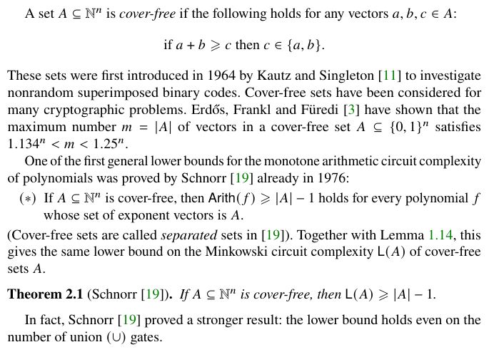
Theorem:
The minimal number of $\min$ or $\max$ gates in a
tropical $(\min,+)$ or $(\max,+)$ circuit computing the tropical $n$-degree convolution is $n^2-2n+1$.
Proof:
We prove the theorem for $(\min,+)$ circuits; the proof for $(\max,+)$ circuits is the same with $\min$ replaced by $\max$.
Consider the
sum-polynomial
\[
SP(x,y)=\sum_{k=0}^{2n-2} z_{k}\cdot P_k(x,y)
= \sum_{k=0}^{2n-2} \sum_{i=0}^k x_iy_{k-i}z_k
\]
of the (arithmetic) $n$-degree convolution, where $z_0,\ldots,z_{2n-2}$ are new $2n-1$ variables.
Let $A$ be the set of all $|A|=n^2$ exponent vectors of the sum-polynomial $SP$.
Every
monomial $ x_iy_{k-i}z_k$ of $SP$ is uniquely determined by
any two its variables. So, the set $A$ is cover-free, and
Schnorr's theorem (Theorem 2.1(1)) implies that every Minkowski $(\cup,+)$ circuit
producing the set $A$ must have at least $|A|-1=n^2-1$ union $(\cup)$ gates.
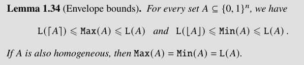
Since the set $A$ is homogeneous (of degree $3$),
Lemma 1.34(2) yields the same lower bound $n^2-1$ on
the number of $\min$ gates in every $(\min,+)$ circuit computing the tropical $(\min,+)$ version
\[
ST(x,y,z)= \min\Big\{x_i+y_{k-i}+z_k\colon k=0,1,\ldots, 2n-2 \mbox{ and } i=0,1,\ldots,k\Big\}
\]
of the sum-polynomial $SP$.
Now, given a $(\min,+)$ circuit for the $(\min,+)$ version $T=\{T_0,T_1,\ldots,T_{2n-2}\}$ of the $n$-degree convolution, we can solve $ST$ by adding
$2n-2$ additional $\min$ gates. Thus, the number of $\min$ gates in every $(\min,+)$ circuit computing $T$ is at least $(n^2-1)-(2n-2)=n^2-2n+1$.
∎
Footnotes:
(1)
 Jump back ☝
(2)
 Jump back ☝
References:
- Schnorr, C.P.: A lower bound on the number of additions in monotone computations. Theor.
Comput. Sci. 2(3), 305–315 (1976) Local copy
⇦ Back to the comments page