\( \def\<#1>{\left<#1\right>} \let\geq\geqslant \let\leq\leqslant % an undirected version of \rightarrow: \newcommand{\mathdash}{\relbar\mkern-9mu\relbar} \def\deg#1{\mathrm{deg}(#1)} \newcommand{\dg}[1]{d_{#1}} \newcommand{\Norm}{\mathrm{N}} \newcommand{\const}[1]{c_{#1}} \newcommand{\cconst}[1]{\alpha_{#1}} \newcommand{\Exp}[1]{E_{#1}} \newcommand*{\ppr}{\mathbin{\ensuremath{\otimes}}} \newcommand*{\su}{\mathbin{\ensuremath{\oplus}}} \newcommand{\nulis}{\vmathbb{0}} %{\mathbf{0}} \newcommand{\vienas}{\vmathbb{1}} \newcommand{\Up}[1]{#1^{\uparrow}} %{#1^{\vartriangle}} \newcommand{\Down}[1]{#1^{\downarrow}} %{#1^{\triangledown}} \newcommand{\lant}[1]{#1_{\mathrm{la}}} % lower antichain \newcommand{\uant}[1]{#1_{\mathrm{ua}}} % upper antichain \newcommand{\skal}[1]{\langle #1\rangle} \newcommand{\NN}{\mathbb{N}} % natural numbers \newcommand{\RR}{\mathbb{R}} \newcommand{\minTrop}{\mathbb{T}_{\mbox{\rm\footnotesize min}}} \newcommand{\maxTrop}{\mathbb{T}_{\mbox{\rm\footnotesize max}}} \newcommand{\FF}{\mathbb{F}} \newcommand{\pRR}{\mathbb{R}_{\mbox{\tiny $+$}}} \newcommand{\QQ}{\mathbb{Q}} \newcommand{\ZZ}{\mathbb{Z}} \newcommand{\gf}[1]{GF(#1)} \newcommand{\conv}[1]{\mathrm{Conv}(#1)} \newcommand{\vvec}[2]{\vec{#1}_{#2}} \newcommand{\f}{{\mathcal F}} \newcommand{\h}{{\mathcal H}} \newcommand{\A}{{\mathcal A}} \newcommand{\B}{{\mathcal B}} \newcommand{\C}{{\mathcal C}} \newcommand{\R}{{\mathcal R}} \newcommand{\MPS}[1]{f_{#1}} % matrix multiplication \newcommand{\ddeg}[2]{\#_{#2}(#1)} \newcommand{\length}[1]{|#1|} \DeclareMathOperator{\support}{sup} \newcommand{\supp}[1]{\support(#1)} \DeclareMathOperator{\Support}{sup} \newcommand{\spp}{\Support} \newcommand{\Supp}[1]{\mathrm{Sup}(#1)} %{\mathcal{S}_{#1}} \newcommand{\lenv}[1]{\lfloor #1\rfloor} \newcommand{\henv}[1]{\lceil#1\rceil} \newcommand{\homm}[2]{{#1}^{\langle #2\rangle}} \let\daug\odot \let\suma\oplus \newcommand{\compl}[1]{Y_{#1}} \newcommand{\pr}[1]{X_{#1}} \newcommand{\xcompl}[1]{Y'_{#1}} \newcommand{\xpr}[1]{X'_{#1}} \newcommand{\cont}[1]{A_{#1}} % content \def\fontas#1{\mathsf{#1}} %{\mathrm{#1}} %{\mathtt{#1}} % \newcommand{\arithm}[1]{\fontas{Arith}(#1)} \newcommand{\Bool}[1]{\fontas{Bool}(#1)} \newcommand{\linBool}[1]{\fontas{Bool}_{\mathrm{lin}}(#1)} \newcommand{\rBool}[2]{\fontas{Bool}_{#2}(#1)} \newcommand{\BBool}[2]{\fontas{Bool}_{#2}(#1)} \newcommand{\MMin}[1]{\fontas{Min}(#1)} \newcommand{\MMax}[1]{\fontas{Max}(#1)} \newcommand{\negMin}[1]{\fontas{Min}^{-}(#1)} \newcommand{\negMax}[1]{\fontas{Max}^{-}(#1)} \newcommand{\Min}[2]{\fontas{Min}_{#2}(#1)} \newcommand{\Max}[2]{\fontas{Max}_{#2}(#1)} \newcommand{\convUn}[1]{\fontas{L}_{\ast}(#1)} \newcommand{\Un}[1]{\fontas{L}(#1)} \newcommand{\kUn}[2]{\fontas{L}_{#2}(#1)} \newcommand{\Nor}{\mu} % norm without argument \newcommand{\nor}[1]{\Nor(#1)} \newcommand{\bool}[1]{\hat{#1}} % Boolean version of f \newcommand{\bphi}{\phi} % boolean circuit \newcommand{\xf}{\boldsymbol{\mathcal{F}}} \newcommand{\euler}{\mathrm{e}} \newcommand{\ee}{f} % other element \newcommand{\exchange}[3]{{#1}-{#2}+{#3}} \newcommand{\dist}[2]{{#2}[#1]} \newcommand{\Dist}[1]{\mathrm{dist}(#1)} \newcommand{\mdist}[2]{\dist{#1}{#2}} % min-max dist. \newcommand{\matching}{\mathcal{M}} \renewcommand{\E}{A} \newcommand{\F}{\mathcal{F}} \newcommand{\set}{W} \newcommand{\Deg}[1]{\mathrm{deg}(#1)} \newcommand{\mtree}{MST} \newcommand{\stree}{{\cal T}} \newcommand{\dstree}{\vec{\cal T}} \newcommand{\Rich}{U_0} \newcommand{\Prob}[1]{\ensuremath{\mathrm{Pr}\left\{{#1}\right\}}} \newcommand{\xI}{\boldsymbol{I}} \newcommand{\plus}{\mbox{\tiny $+$}} \newcommand{\sgn}[1]{\left[#1\right]} \newcommand{\ccompl}[1]{{#1}^*} \newcommand{\contr}[1]{[#1]} \newcommand{\harm}[2]{{#1}\,\#\,{#2}} %{{#1}\,\oplus\,{#2}} \newcommand{\hharm}{\#} %{\oplus} \newcommand{\rec}[1]{1/#1} \newcommand{\rrec}[1]{{#1}^{-1}} \DeclareRobustCommand{\bigO}{% \text{\usefont{OMS}{cmsy}{m}{n}O}} \newcommand{\dalyba}{/}%{\oslash} \newcommand{\mmax}{\mbox{\tiny $\max$}} \newcommand{\thr}[2]{\mathrm{Th}^{#1}_{#2}} \newcommand{\rectbound}{h} \newcommand{\pol}[3]{\sum_{#1\in #2}{#3}_{#1}\prod_{i=1}^n x_i^{#1_i}} \newcommand{\tpol}[2]{\min_{#1\in #2}\left\{\skal{#1,x}+\const{#1}\right\}} \newcommand{\comp}{\circ} % composition \newcommand{\0}{\vec{0}} \newcommand{\drops}[1]{\tau(#1)} \newcommand{\HY}[2]{F^{#2}_{#1}} \newcommand{\hy}[1]{f_{#1}} \newcommand{\hh}{h} \newcommand{\hymin}[1]{f_{#1}^{\mathrm{min}}} \newcommand{\hymax}[1]{f_{#1}^{\mathrm{max}}} \newcommand{\ebound}[2]{\partial_{#2}(#1)} \newcommand{\Lpure}{L_{\mathrm{pure}}} \newcommand{\Vpure}{V_{\mathrm{pure}}} \newcommand{\Lred}{L_1} %L_{\mathrm{red}}} \newcommand{\Lblue}{L_0} %{L_{\mathrm{blue}}} \newcommand{\epr}[1]{z_{#1}} \newcommand{\wCut}[1]{w(#1)} \newcommand{\cut}[2]{w_{#2}(#1)} \newcommand{\Length}[1]{l(#1)} \newcommand{\Sup}[1]{\mathrm{Sup}(#1)} \newcommand{\ddist}[1]{d_{#1}} \newcommand{\sym}[2]{S_{#1,#2}} \newcommand{\minsum}[2]{\mathrm{MinS}^{#1}_{#2}} \newcommand{\maxsum}[2]{\mathrm{MaxS}^{#1}_{#2}} % top k-of-n function \newcommand{\cirsel}[2]{\Phi^{#1}_{#2}} % its circuit \newcommand{\sel}[2]{\sym{#1}{#2}} % symmetric pol. \newcommand{\cf}[1]{{#1}^{o}} \newcommand{\Item}[1]{\item[\mbox{\rm (#1)}]} % item in roman \newcommand{\bbar}[1]{\underline{#1}} \newcommand{\Narrow}[1]{\mathrm{Narrow}(#1)} \newcommand{\Wide}[1]{\mathrm{Wide}(#1)} \newcommand{\eepsil}{\varepsilon} \newcommand{\amir}{\varphi} \newcommand{\mon}[1]{\mathrm{mon}(#1)} \newcommand{\mmon}{\alpha} \newcommand{\gmon}{\alpha} \newcommand{\hmon}{\beta} \newcommand{\nnor}[1]{\|#1\|} \newcommand{\inorm}[1]{\left\|#1\right\|_{\mbox{\tiny $\infty$}}} \newcommand{\mstbound}{\gamma} \newcommand{\coset}[1]{\textup{co-}{#1}} \newcommand{\spol}[1]{\mathrm{ST}_{#1}} \newcommand{\cayley}[1]{\mathrm{C}_{#1}} \newcommand{\SQUARE}[1]{\mathrm{SQ}_{#1}} \newcommand{\STCONN}[1]{\mathrm{STCON}_{#1}} \newcommand{\STPATH}[1]{\mathrm{PATH}_{#1}} \newcommand{\SSSP}[1]{\mathrm{SSSP}(#1)} \newcommand{\APSP}[1]{\mathrm{APSP}(#1)} \newcommand{\MP}[1]{\mathrm{MP}_{#1}} \newcommand{\CONN}[1]{\mathrm{CONN}_{#1}} \newcommand{\PERM}[1]{\mathrm{PER}_{#1}} \newcommand{\mst}[2]{\tau_{#1}(#2)} \newcommand{\MST}[1]{\mathrm{MST}_{#1}} \newcommand{\MIS}{\mathrm{MIS}} \newcommand{\dtree}{\mathrm{DST}} \newcommand{\DST}[1]{\dtree_{#1}} \newcommand{\CLIQUE}[2]{\mathrm{CL}_{#1,#2}} \newcommand{\ISOL}[1]{\mathrm{ISOL}_{#1}} \newcommand{\POL}[1]{\mathrm{POL}_{#1}} \newcommand{\ST}[1]{\ptree_{#1}} \newcommand{\Per}[1]{\mathrm{per}_{#1}} \newcommand{\PM}{\mathrm{PM}} \newcommand{\error}{\epsilon} \newcommand{\PI}[1]{A_{#1}} \newcommand{\Low}[1]{A_{#1}} \newcommand{\node}[1]{v_{#1}} \newcommand{\BF}[2]{W_{#2}[#1]} % Bellman-Ford \newcommand{\FW}[3]{W_{#1}[#2,#3]} % Floyd-Washall \newcommand{\HK}[1]{W[#1]} % Held-Karp \newcommand{\WW}[1]{W[#1]} \newcommand{\pWW}[1]{W^{+}[#1]} \newcommand{\nWW}[1]{W^-[#1]} \newcommand{\knap}[2]{W_{#2}[#1]} \newcommand{\Cut}[1]{w(#1)} \newcommand{\size}[1]{\mathrm{size}(#1)} \newcommand{\dual}[1]{{#1}^{\ast}} \def\gcd#1{\mathrm{gcd}(#1)} \)
[This is a supplementary material to Chapter 5, Section 5.3]

Bellman-Ford-Moore (min,+) branching program for lightest k-walks is optimal

Recall that a tropical $(\min,+)$ branching program $\Phi$ is a directed acyclic graph with one zero indegree node $s$ (the source node) and one zero outdegree node $t$ (the target node). Programs simultaneously computing several functions may have several target nodes. Multiple edges joining the same pair of nodes are allowed. Every edge is either labeled by one of the variables 
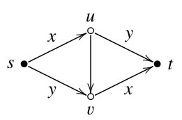
$x_1,\ldots,x_n$ (is a switch) or is unlabeled (is a rectifier). The minimization problem solved by $\Phi$ is the minimum, over all $s$-$t$ paths $\pi$ in $\Phi$, of the sum of labels of the edges along the path $\pi$ (see Fig. 1).
Branching program Fig. 1: A $(\min,+)$ branching program with four switches and one rectifier (from $u$ to $v$) solving the minimization problem $f(x,y)=\min\{2x, x+y\}$.

As before, let $K_n$ be the complete undirected graph on $[n]=\{1,\ldots,n\}$. The length of a walk in $K_n$ is the number of its edges; if an edge is traversed several times during the walk, then this edge is counted this number of times. In the lightest $k$-walk problem, given an assignment of nonnegative weights $x_{i,j}$ to the edges $\{i,j\}$ of $K_n$, the goal is to compute the minimum weight \[ x_{1,i_1} + x_{i_1,i_2}+ x_{i_2,i_3}+\cdots + x_{i_{k-2},i_{k-1}}+x_{i_{k-1},n} \] of a walk $(s,i_1,i_2,\ldots,i_{k-1},t)$ of length $k$ between the vertices $1$ and $n$, where $i_j\neq i_{j+1}$ for all $j=1,\ldots,k-2$ (variables $x_{i,j}$ correspond to the edges $\{i,j\}$ of $K_n$), but $\{i_j,i_{j+1}\}=\{i_l,i_{l+1}\}$ for $j\neq l$ is possible, that is, one can walk through the same edge several times. 
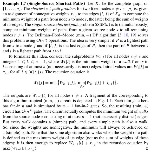
The lightest $k$-walk problem on $K_n$ can be solved by a $(\min,+)$ branching program with at most $kn^2$ switches using the Bellman-Ford-Moore $(\min,+)$ DP algorithm (Example 1.7(1)).

The BFM $(\min,+)$ branching program: We have one source node $s=1$, one target node $t=n$, and $k-1$ intermediate layers of nodes $V_1,V_2,\ldots,V_{k-1}$ with $|V_2|=\ldots=|V_{k}|=n-2$, each of which is a copy of nodes $\{2,\ldots,n-1\}$: \[ s \Rightarrow V_1 \Rightarrow V_2 \Rightarrow \cdots \Rightarrow V_{k-1} \Rightarrow t\,. \] Edges go only from one layer to the next layer. The edge going from the source node $s$ to the $i$-th node on the fist layer $V_1$ is a switch labeled by the variable $x_{s,i}$, and the edge going from the $i$-th node in the last layer $V_{k-1}$ to the target node $t$ is also a switch labeled by the variable $x_{i,t}$. For every $i\neq j\in \{2,\ldots,n-1\}$, the $j$-th node on the $(l+1)$-th layer $V_{l+1}$ is entered by a switch from the $i$-th node on the previous $l$-th layer $V_{l}$ and is labeled with the variable $x_{i,j}$. The resulting branching program has $\leq kn^2$ switches in total.      $\Box$

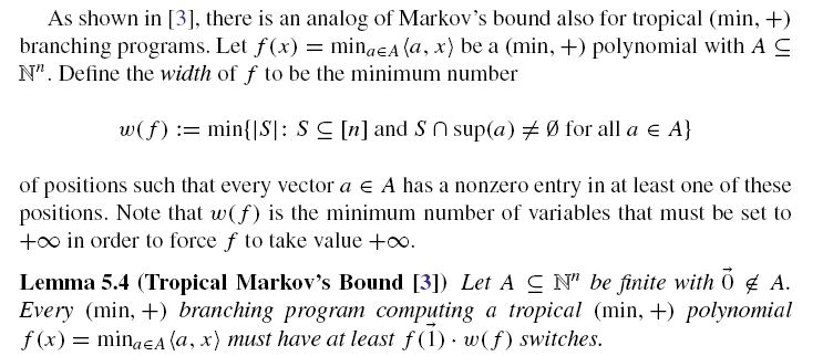
The following consequence of tropical Markov's bound (Lemma 4.4(2)) shows that this tropical $(\min,+)$ branching program is essentially optimal (among all such branching programs for this problem).

Theorem A Let $4\leq k\leq n-2$. Every $(\min,+)$ branching program solving the lightest $k$-walk problem on $K_n$ must have at least a constant times $kn(n-k)$ switches.
Proof We will use the following classical result of Erdős and Gallai [1]: for $l\geq 1$, every $m$-vertex graph with $\gt (l-1)m/2$ edges contains a path of length $l$. Since $\binom{m}{2}-(l-1)m/2=m(m-l)/2$, this result can be re-stated as:
Note that this bound cannot be improved. Indeed, if $m=ql$ is a multiple of $l$, then we can split the vertices of $K_m$ into $q$ disjoint sets of size $l$, and remove all edges lying between these sets. The resulting graph has no paths of length $l$, and we have removed only $\binom{q}{2}l^2=m(m-l)/2$ edges.

Now consider the minimization problem \begin{equation}\label{eq:walk1} f(x)= \min \left\{ x_{i_1,i_2}+ x_{i_2,i_3}+\cdots + x_{i_{k-2},i_{k-1}}\right\}\,, \end{equation} where the minimum is over all walks $(i_1,\ldots,i_{k-1})$ of length $l:=k-2$ in the complete graph $K_m$ on $m:=n-2$ nodes $\{2,\ldots,n-1\}$. The problem $f$ is a subproblem of the lightest $k$-walk problem when all $2(n-1)$ edges of $K_n$ incident with the vertex $1$ or with the vertex $n$ of $K_n$ are given zero weight. It is thus enough to prove that every $(\min,+)$ branching program solving the problem $f$ must have at least a constant times $kn(n-k)$ switches.

We clearly have $f(\vec{1})\geq k-2$. To lower bound the width $\Cut{f}$ of $f$, let $Y$ be a set of $|Y|=\Cut{f}$ variables of $f$ such that every sum of $f$ contains at least one of these variables. Every path of length $l$ in $K_m$ is also a walk of length $l$. So, for every path of length $l$ in $K_m$, there is a sum in Eq. \eqref{eq:walk1} whose variables correspond to the edges of that path. Thus, this sum must contain at least one variable in $Y$. This means that removal from $K_m$ of all edges corresponding to the variables in $Y$ destroys all paths of length $l$ in $K_m$. The Erdős-Gallai result gives $\Cut{f}=|Y|\geq m(m-l)/2= (n-2)(n-k)/2$. Since $f(\vec{1})\geq k-2$, Lemma 5.4(1) implies that every branching program computing $f$ over the $(\min,+)$ semiring must have at least $f(\vec{1})\cdot \Cut{f}$ switches, which is at least a constant times $kn(n-k)$.

Remark 1: Note that a slight modification of the BFM $(\min,+)$ branching program for the lightest $k$-walk problem can also solve the lightest $s$-$t$ path problem in $K_n$: just set $k:=n$ and add rectifiers (non-labeled edges) between the $i$th node in one layer $V_l$ to the $i$th node in the next layer $V_{l+1}$. The resulting branching program(3) has only $O(n^3)$ switches. Whether this branching program is also optimal among all $(\min,+)$ branching programs for the lightest $s$-$t$ path problem remains, however, an open problem: the argument we used in the proof of Theorem A (based on the Erdős-Gallai result) does not work then anymore.      $\Box$

Remark 2: 
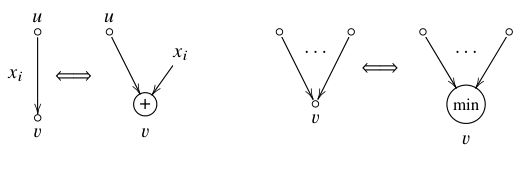
Tropical branching programs $\Phi$ correspond to so-called skew tropical circuits $\Phi'$ where one of the two inputs to each addition $(+)$ gate is a variable. Namely, every switch $(u,v)$ in $\Phi$ labeled by a variable $x_i$ as an addition gate $v=u+x_i$ in $\Phi'$, every rectifier $(u,v)$ (unlabeled edge) in $\Phi$ as addition gate $v=u+0$ in $\Phi'$; since such gates are fully redundant, we can assume that such gates are not present in $\Phi'$. Every node $v$ in $\Phi$ is a gate in $\Phi'$ performing a min or max operation:

Circuits to BPs
Thus, the number of switches in $\Phi$ is exactly the number of addition $(+)$ gates in the skew circuit $\Phi'$, while (unbounded fanin) $\min$ or $\max$ gates are "for free".      $\Box$
Footnotes:

(1)   Jump back ☝


(2)   Jump back ☝
(3)   Jump back ☝

References:

  1. P. Erdős and T. Gallai: On maximal paths and circuits in graphs, Acta Math. Acad. Sci. Hungar., 10 (1959) 337-356.   Local copy


⇦   Back to the comments page